Coriolis Force

Bastien_Delacroix · November 12, 2018, 9:00pm

Dear LAMMPS users,

The problem:
I would like to model a particle in rotation around an axis. But I
would like to resolve my problem in the rotating frame. That’s why I
must add some inertial forces to my particle:
-Centrifugal Force (F=w*w*R)
-Coriolis Force (F=-2*W X v) with v the velocity vector and W the axis vector
To do this I created two new fix command for each force. My fixes have
the mask post_force and I add my new forces in the post_force function.

The question:
Is it correct to do this add in the post_force function? (The
Coriolis force depend on the velocity of the particle, so I wonder if
it is correct to do this here.)

Why this question?
I did a test case with a particle subjected to no force (without any
contacts and without gravity) except the Coriolis and Centrifugal
Force. Thus, the expected trajectory of the particle is a circle in
the rotating frame. But I obtain a divergence of the trajectory; the
particle is moving away from the center. (The trajectory is like a
snail)

So, I wonder what is the good method to add such force in a model?

Regards,
Bastien Delacroix

akohlmey · November 13, 2018, 12:13am

Dear LAMMPS users,

The problem:
I would like to model a particle in rotation around an axis. But I
would like to resolve my problem in the rotating frame. That’s why I
must add some inertial forces to my particle:
-Centrifugal Force (F=wwR)
-Coriolis Force (F=-2*W X v) with v the velocity vector and W the axis vector
To do this I created two new fix command for each force. My fixes have
the mask post_force and I add my new forces in the post_force function.

The question:
Is it correct to do this add in the post_force function? (The
Coriolis force depend on the velocity of the particle, so I wonder if
it is correct to do this here.)

yes, and no.

since LAMMPS does Velocity Verlet time stepping, you would have to add (half of) the velocity dependent force before the first half velocity update and then again in Fix::post_force() before the second half velocity update. the difference is usually small (the same applies, e.g., to DPD and LAMMPS computes velocity dependent forces only in the dpd pair style, which is equivalent to Fix::post_force. i am not 100% certain, but it might work to do the first (half) force addition during Fix::end_of_step() and then another during Fix::post_force(). i suggest you create some tiny test system with simple fix nve time integration and check it out.
axel.

Stefan_Paquay · November 13, 2018, 12:28am

Somehow I don’t think doing MD in a non-inertial frame is a good idea. If constraining particles to a cylinder or something will solve your problem, take a look at USER-MANIFOLD. Otherwise other people might have some ideas.

_Diaz_Adrian · November 13, 2018, 12:41am

I’m not so sure the system would be stable either physically or numerically with such a force; this may be the cause of the spiral you see. A velocity dependent force, I think, diverges from the Hamiltonian description of the problem and velocity verlet is tailored as a symplectic integrator that bounds the error in energy. I may be wrong though since that’s me dredging old knowledge.

akohlmey · November 13, 2018, 2:59am

Dear LAMMPS users,

The problem:
I would like to model a particle in rotation around an axis. But I
would like to resolve my problem in the rotating frame. That’s why I
must add some inertial forces to my particle:
-Centrifugal Force (F=wwR)
-Coriolis Force (F=-2*W X v) with v the velocity vector and W the axis vector
To do this I created two new fix command for each force. My fixes have
the mask post_force and I add my new forces in the post_force function.

The question:
Is it correct to do this add in the post_force function? (The
Coriolis force depend on the velocity of the particle, so I wonder if
it is correct to do this here.)

Why this question?
I did a test case with a particle subjected to no force (without any
contacts and without gravity) except the Coriolis and Centrifugal
Force. Thus, the expected trajectory of the particle is a circle in
the rotating frame. But I obtain a divergence of the trajectory; the
particle is moving away from the center. (The trajectory is like a
snail)

why is this wrong?

the centrifugal force should push the particle away from the center (unless it is exactly in the center, where there is no force and thus no motion) and the coriolis force should push the particle sideways orthogonal to that, and the resulting trajectory would be a spiral.

axel.

Bastien_Delacroix · November 15, 2018, 10:50pm

Thanks you for you very helpful answer,
To precise my subject I work in DEM and I hope that it is possible to work in rotating frame.
Firstly, I would like to expose my vision about a circular trajectory. If we have a fix particle in the Eulerian frame, from my point of view, this particle will have a circular trajectory in the Lagrangian frame because there is only a difference angular velocity between these two frames and my particle is no subjected to external force. But I agree with your explanation too, so I am a bit lost. It is a very important question for me because it can be the source of my mistakes. So, I will be very thankful if you have the right answer.
For the integration I tried what you suggest about the separation of the Coriolis force in the fix:: post_force and in the fix::end_of_step. Unfortunately, it seems that it doesn’t work (in the hypothesis of a circular trajectory). I have a new spiral but it is more expanded.
Regards
Bastien Delacroix

Axel Kohlmeyer <[email protected]> a écrit :

Eric_Murphy1 · November 16, 2018, 4:44am

I think it should obvious that in a physical system you should not get a spiral in a rotating frame, if a particle is standing still in the non-inertial frame.

This seems trivially settled by just writing a small python script and computing - to test if nothing else your understanding. As I have done below with the correct forms of the forces. I also included some trajectories (an artifact of what I’m talking about) - as you should do in the future so discussions can be productive. The trajectory is fairly circular with a small enough time-step for the trajectory, but does indeed travel outwards in a spiral that tightens the smaller you choose the time-step. I would lean towards what Adrian describes in this set-up being numerically unstable.

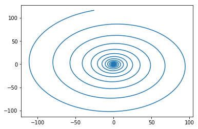
I show 3 cases each run for the same amount of numerical time (they are shown in order) - all should go ~16 revolutions

time step = 0.01; steps = 10^4 (radial position ~100X larger than the correct answer)
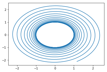
time step = 0.001; steps = 10^5 (radial position about 100% error)
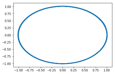
time step = 0.0001; steps = 10^6 (gives ~ 2% error in the radial position)

This situation seems ripe for instability with two forces that must intimately balance one another with one essentially depending on the magnitude of the position (centrifugal) and the magnitude of the velocity (Coriolis). At a very basic level, having force evaluations where position (\propto centrifugal repulsive force) is a half step ahead of the velocity (\propto Coriolis attractive force) might be cause for concern and a growing numerical instability.

However… Ultimately, you’ll be performing DEM. I assume you’ll be bounding your domain and you’ve got some rotating piece of machinery - otherwise why do it. Given that granular potentials and walls are quite dissipative, frictional, and normally have plenty of contacts, you might not even care about this issue - as long as your time-step is small enough. On top of that a comparison of the time-scales of your granular interactions and those required for getting reasonably stable behavior in your rotating frame (over some large time span) might very well show that the instability it not of much concern for industrially relevant problems.

HTH.

import numpy as np
import matplotlib.pyplot as plt

def Calc_Centrifugal_Accel(angular_velocity,position):
f_cent = -np.cross(angular_velocity,np.cross(angular_velocity,position))

return f_cent

def Calc_Coriolis_Accel(angular_velocity, velocity):
f_cor = -2.*np.cross(angular_velocity,velocity)

return f_cor

assumes we rotate about the origin

axis_of_rotation = np.array([0,0,1])
angular_speed = 1
angular_velocity = angular_speed*axis_of_rotation

position = np.zeros((1,3))
position[0,0] = 1

initial velocity of the particle is in the opposite direction

of the tangential velocity of the frame at that point

velocity = -np.sign(angular_speed)*np.cross( angular_velocity ,position)
pos = position

a_cent = Calc_Centrifugal_Accel(angular_velocity, position)
a_cor = Calc_Coriolis_Accel(angular_velocity, velocity)
print(a_cent, a_cor)

delt = 0.0001

perform velocity verlet integration on the particle

for i in range(1000000):
a_cent = Calc_Centrifugal_Accel(angular_velocity, position)
a_cor = Calc_Coriolis_Accel(angular_velocity, velocity)
vhalf = velocity + 0.5*(a_cent + a_cor)delt
position = position + vhalfdelt
a_cent = Calc_Centrifugal_Accel(angular_velocity, position)
a_cor = Calc_Coriolis_Accel(angular_velocity, vhalf)
velocity = vhalf + 0.5*(a_cent + a_cor)*delt
#print(np.linalg.norm(position), np.arctan2(position[0,0], position[0,1]), np.linalg.norm(velocity))
pos = np.append(pos, position, axis=0)

plt.plot(pos[:,0],pos[:,1])

Regards,
Eric Murphy, PhD
Multiphase Flow Scientist
Mechanical Engineer
murphyericjames@…24… | 563-449-6661

LinkedIn | ResearchGate | Google Scholar