I want to reproduce a plot for the autocorrelation function (ACF) versus time. As you know, the ACF plot starts at 1 at t=0 and finally vanishes to zero at long times. I used fix ave/correlate as follows:
fix SS H2O ave/correlate 20 5000 100000 &
v_pxycyl v_pxzcyl v_pyzcyl v_pxxcyl v_pyycyl v_pzzcyl type auto file S0St.dat ave running
where v_pxycyl is the stress tensor.
But the bad thing, when I plot the column 2 versus column ($4+$5+$6+$7+$8+$9), I get a large number for ACF (not 1).
The ACF values from ave/correlate ar not normalized as far as I know. You have to do it yourself. The value you get at t=0 is an average of your squared value. Not 1. See the doc page of the fix for more information.
Why do you expect a value starting at one when summing values that you all expect to start at 1? This seems bogus to me. Also a proper way to get the ACF of the sum of all your values would be to compute the ACF of the sum in the fix, not summing the ACF values. I don’t think the operations are commutable.
Last, from a physics point of view, I don’t understand what you are trying to compute. This reminds me a bit of the shear modulus of polymer but the formula would be different.
Thanks for your comments.
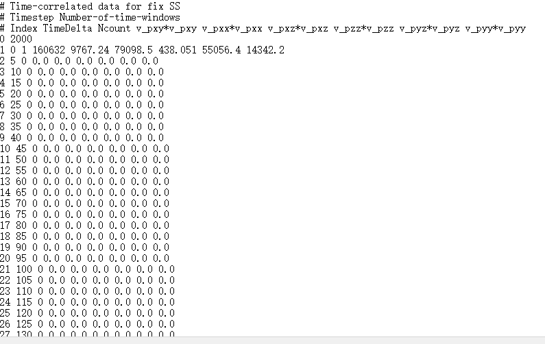
I have calculated stress tensor usingcompute stress/atom. Then, in order to get the ACF, I used fix ave/correlate. A part of my fix ave/correlate results as follows:
The question is about how to use the output of fix ave/correlate data to plot ACF versus time. Should I use any postprocessing program to get ACF of produced fix ave/correlate data??
I got confused how to use the fix ave/correlate data to plot the ACF.
I puzzled over this until it clicked: what statistical physicists call a “time correlation function”, which is \langle A(t) A(0)\rangle for some observable A observed at two time points along one trajectory, is what statisticians call an autocovariance. fix ave/correlate is named for the physicist’s correlation function.
The physicist’s correlation function is not the statistician’s autocorrelation, and so – unless you are doing a purely statistical analysis, such as determining sampling efficiency – you shouldn’t really think in terms of the “ACF”. (After all, autocorrelations are unitless, so how could you get a physical quantity from them without bringing units back in from somewhere?)
As to how to use the correlation function, calculating linear response coefficients from (asymptotic) correlation integrals is known as the Green-Kubo theorem or method, and it is a standard topic of any advanced statistical mechanics textbook.
Hi,do you know how to plot autocorrelation vs time ,I also use fix ave/correlate in order to calculate Thermal conductivity with GK method.I still do not know the file that generated by fix ave/correlate how to use.I read many articles they all plot the autocorrelate vs time .Can you teach me ,thanks
In the future, please do not post after a thread that has been off for several month and open a new conversation dedicated to your issue.
Without more information I can only tell you that the file produced by the fix is indicated as an argument after the file keyword. Please have a look at the documentation for more information on its format.
There are a lot of plotting tools such as Gnuplot, Matplotlib or even Excel and the LibreOffice suite. The format of the file should make it straightforward to plot in one or the other of these softwares.
I’m sorry for that.In actually, I was used GK method to calculate Thermo Conductivity,I read the artical http://dx.doi.org/10.12943/CNR.2018.00009 one more time,when I balance my system, I use fix ave/correlate command to calculate autocorrelation in NVE ensemble,among them, my s p d is 20,3000,60000,my run step is 60000*10,It doesn’t necessarily make sense, I just want to run the process,and I get a file named profile.gk,I think this file is helpful to get autocorrelation,but I’m not clearly how to deal with it. Every 60,000 times 3,000 pieces of data are output.
I suggest you re-read carefully the documentation page I linked previously as it describes how the output file will be formatted, depending on the keywords you use in your command.
There are several ways to do the averaging and write the output. By default, the last averaging done is appended to the end of the file. So you have an array of size N\times{}M where N is your number of values and M the number of time-windows. These values are written every 60000 step in your case. So you should have 10 of them in your file by the end of the simulation, each of them taking 2000 lines. The values are initially set to 0 so this explains the head of of your output file. Depending on your settings, the following data blocks can be individual correlations averaging or a running average that is updated and written regularly. Both of these cases would require different post-processing strategies.
In the future, as suggested, do not hesitate to start a new topic with a clear title related to your issue, instead of replying in this one.
Hi,Germain! I’m sorry I saw your reply after so long, I read the fix ave/correlate command again and I don’t know if my understanding was correct. For example, fix ave/correlate 20 3000 60000 value1 value2 value3 type auto file profile.gk ave running,run 6000010, then my profile.gk file is in the following form: 0 3000; 60000 3000; 12000 3000; up to 6000010 3000; There will be 11 of them in total, each with 3000 lines in my profile.gk file. Do I not need to care about the 3000 rows of data below 0 3000, but start from 60000 3000 and go all the way to 6000010 3000. I averaged the data from 60000 3000 and every subsequent row in the profile.gk file, i.e. (b1+b2+b3)/3, (because I only found the autocorrelation of value1,2,3). Then, for example, 60000 3000, 120000 3000 until 6000010 3000 in the average of the corresponding rows averaged again, that is, (a1+a2+…+a10)/10, you can get the autocorrelation function vs time data points (a total of 3000 data points), if I want to normalize, divide the data points by the first one, am my understanding correct? I still have a question, that is, 0 What’s the point of the data below 3000, or what does it do? I’m confused