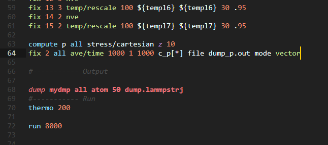
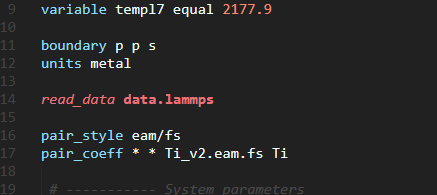
I want to plot the pressure profile with respect to z direction that is the height of the column. I used the compute stress/cartesian command as shown in the following code:
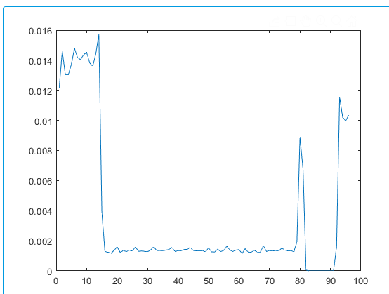
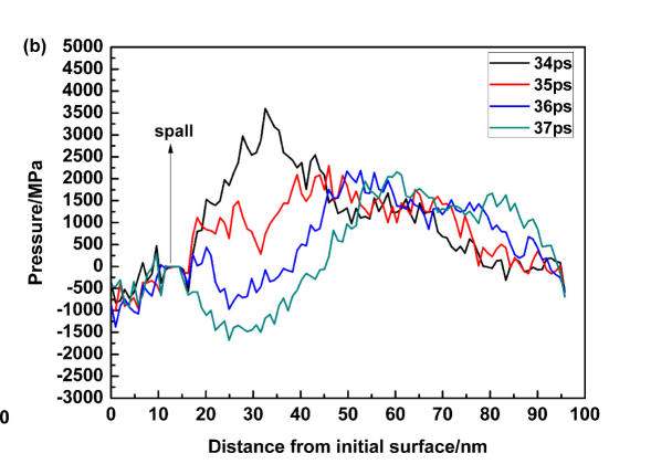
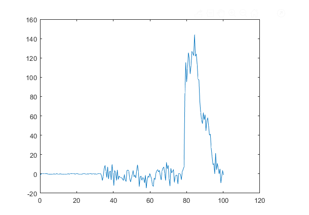
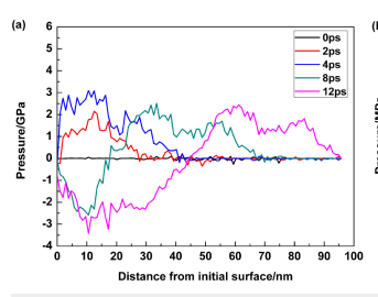
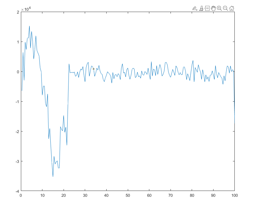
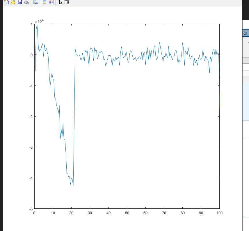
when the generated data is plotted it does not match the expected result. For example at 7000 time steps or 35 ps the stress distribution with respect to depth along z axis the plot looks like following (I calculated the total pressure by summing the virial and kinetic component of pressure in z axis)
this is not in agreement with known results
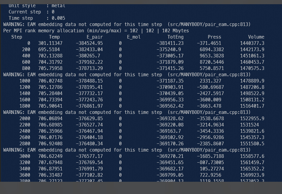
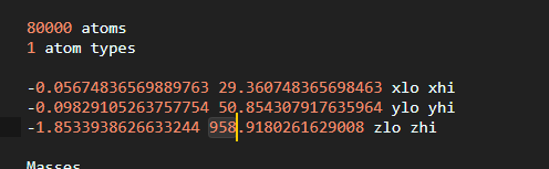
I got this warning when lammps ran
This might be related to the restriction given in documentation that this compute style gives incorrect result for many body pair style and I used an EAM potential for titanium.
My question is how to get the same function of this compute style with many body pair style
Any sort of hint will highly appreciated. Thanks in advance.
There is no other implementation of this kind of compute in LAMMPS for the same geometry.
But to compute a pressure/stress profile this is not needed. If I remember correctly, the compute you are using is specifically meant to be used for liquids.
Instead what you can do is use compute stress/atom, and use compute chunk/atom to define a 1d-binning geometry and then compute reduce/chunk to sum the stress components from the atoms into each bin (=chunk) and finally fix ave/chunk to get the average over multiple timesteps. The documentation for compute stress/atom shows how to get the global scalar pressure from the per-atom stress (negative of the average of the per-component sums divided by the volume). You need to adapt that to the volume of your bins.
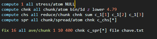
Okay so, This is what I have coded for computing pressure
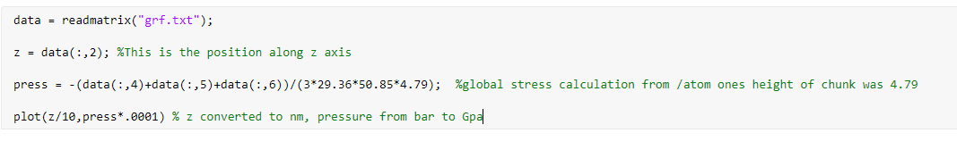
I did the atomic to global stress conversion in matlab (still not confident with doing it in lammps) and plotted the pressure along z coordinates (from the fix ave/chunk output)
I just made some quick test and here is what I came up with:
# set number of bins
variable nbins index 200
variable fraction equal 1.0/v_nbins
# define bins as chunks
compute cchunk all chunk/atom bin/1d x lower ${fraction} units reduced
compute stress all stress/atom NULL
# apply conversion to pressure early since we have no variable style for processing chunks
variable press atom -(c_stress[1]+c_stress[2]+c_stress[3])/(3.0*vol*${fraction})
compute binpress all reduce/chunk cchunk sum v_press
fix avg all ave/time 10 40 400 c_binpress mode vector file ave_stress.txt
The problem of measuring stress is atleast solved. Values are close to the expected result. The trend is just not matching. The paper did not disclose if they had averaged over time.
But can you give some insight to what I should consider when choosing values of Nevery, Nrepeat, Nfreq?? In your code, you used 10 40 400, so averaging is done at 400th step with 40 data at 10 time step interval(correct me if i am wrong). Then the average is over the whole 400 steps timespan.
Since I am focusing on result at certain moment (i.e. 8 ps it is around 1600 steps), shouldn’t I only average over values near that time?
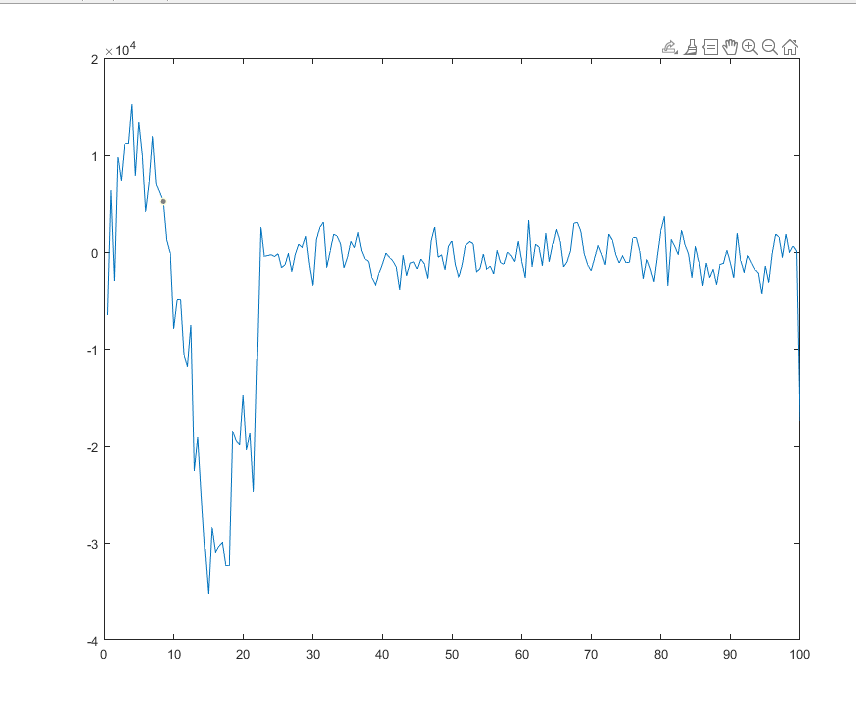
And the step size of the simulation is affecting the plot trend
with 1 femtosecon And
plot:
I guess the problem is in the parameters I am choosing. Just so you know, my supervisor is not exactly from MD background. He is interested to find the mechanism of laser ablation using molecular dynamics and so I venturing this world all on my own.
Could you also give some advice about how to deal with these type of problem (I mean when the issue isnt the code rather the logic)
@Sabik I think you are narrowing down the possible causes for the difference. It could also be caused by other parts of your model. You use of fix temp/rescale seems odd and your use of multiple fix nve instances wasteful (why not just one?).
But how to plan your research and models, is beyond the scope of this forum and has next to nothing to do with LAMMPS (unlike discussing how to extract some property from the simulation). What you are asking for is what is the job of an adviser, so you should discuss with your adviser. I don’t have the time (and interest) to be an (unpaid) adviser on a research project overseen by another (paid) adviser.
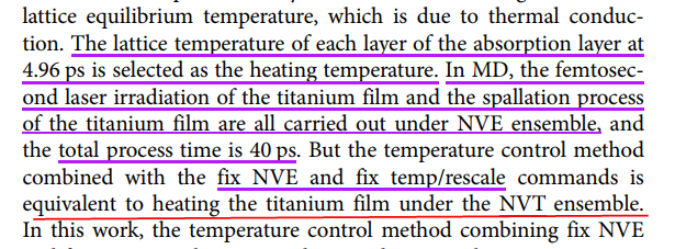
The multiple instaces of fix nvt is based on the paper i am following. They divided the domain in 7 layers and heated each to different temperature found from solving two temperature model
And @akohlmey , what I am aiming for ‘my paper’ is using the ttm in lammps. In the paper mentioned, the ttm equation is solved in matlab pde solver and result is given to lammps at 7 layers. This is okay for simplification. But not accurate. However the ttm in lammps treats the energy as simple heat source. But my supervisor (from an optics background) won’t allow that. Energy deposition from laser is to be solved from wave equation numerically. So the source term needs to adjusted in “fix ttm/mod”.
Simply put, i have to edit the source code. And i have no idea where to start. At least you can give me some useful tips on that regard??
Whoever authored this paper has a dangerously incomplete understanding of statistical mechanics. The statement that fix nve plus fix temp/rescale is equivalent to an NVT ensemble is incorrect. If I had been a reviewer of this paper, these statements alone would be a reason to reject. Using fix temp/rescale for any production calculation is a very, very bad idea. LAMMPS has many alternatives that are better every aspect.
Worrying about accuracy and using fix temp/rescale at the same time is a stark contradiction.
Not much. There is lots of information about modifying LAMMPS and some of its inner workings in the programmer’s guide section of the manual, but beyond that you have to be able to read and understand source code. There is no alternative to it. In the case of fix ttm it is doubly important since there will be few people that understand the physics of the model well enough. I don’t.
This sounds like a case where you should contact the authors of the original paper for further advice. In your position, I would start by simply trying to obtain their input script and data and trying to replicate their result, and then looking at Axel’s script fragment and seeing if it gives results comparable to “stress/cartesian”.
Start with what has been published and make small, incremental changes, validating at each step. “I need to write new source code” can have a very low reward/risk ratio – you owe it to yourself to explore every other possibility first.
You also need to understand the theory you are trying to implement from the ground up. Simulations in a peer reviewed paper can still be misunderstood, misapplied, poorly described, inappropriately initialized, and wrong in many other wonderful and creative ways.
Considering the crudeness of the described model and the apparent lack of experience in statistical mechanics of the authors as evidenced by the quoted excerpt, I would rather advice against following the advice of those authors, but instead look for some other publication by somebody more experienced and paying more attention to the quality of the applied model.