Brownian Dynamics in LAMMPS

Dear Steve and other LAMMPS developers,

I am a first year PhD student, and one of my aspirations is to study polymer dynamics theoretically and computationally, and I plan to use LAMMPS for my simulations. I have worked with the software package before which proved to be very productive, and I plan to continue and use it for my future studies.

I have one general LAMMPS Brownian Dynamics enquiry and 3 specific questions related to the fix_langevin.cpp code, which together with fix_nve (the microcanonical ensemble in which particle number volume and energy are conserved) performs Brownian dynamics.

(1)

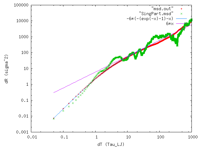
I would like to know if simulations of Brownian motion have been performed with LAMMPS such that they show the diffusion limit <x²> = Dt and fluctuations about it? I have attempted to do this with fix_nve and fix_langevin, however, when I plotted |r²| of my particle vs timestep, the behaviour was not linear as I was expecting (if needed, I can provide the script for this).

(2)

I understand that by fluctuation dissipation theorem, there exists a relation between the strength of stochastic force fluctuations and friction (hydrodynamic drag), which by equipartition can be expressed as: stochastic force intensity = 2*kBT*hydrodynamic drag.

I believe that the FDT is incorporated in the following part of the code:

for (int i = 0; i < nlocal; i++) {
if (mask[i] & groupbit) {
inertiaone = SINERTIA*radius[i]*radius[i]*rmass[i];
gamma1 = -inertiaone / t_period / ftm2v;
gamma2 = sqrt(inertiaone) * sqrt(24.0*boltz/t_period/dt/mvv2e) / ftm2v;

From documentation,

" Magnituge of stochastic force is proportional to sqrt(Kb T m / dt damp), where Kb is the Boltzmann constant, T is the desired temperature, m is the mass of the particle, dt is the timestep size, and damp is the damping factor (this is specified in time units and determines how rapidly the temperature is relaxed and is thought to be inversely related to the viscosity of the solvent). " Could someone possibly clarify the origin of this formulation as I struggle to understand how this equation is derived.

(3)

Also, I cannot quite understand what the following expressions mean, to be more precise, why are gammas assigned and multiplied as 1/ ratios:

gamma1 *= 1.0/ratio[type[i]];
gamma2 *= 1.0/sqrt(ratio[type[i]]) * tsqrt;

(4)

Having read the topics in the mailing list discussion, I understand that the prefactor (24) comes from uniform random number generator. Steve referred to Dunweg et al. when this question was raised before; having read the Dunweg paper (please find attached), I still struggle to understand where this prefactor comes from.

Thank you very much in advance!

With best wishes,
Anna Lappala

PS. Unfortunately, I cannot send the Dunweg article as an attachment to the mail-list as it is too big!

On what timescale are you seeing the nonlinear behavior?

I have just one remark: to clarify the term "Brownian Dynamics". This
means different things to different people.
http://en.wikipedia.org/wiki/Brownian_dynamics
If, as in the wikipedia article, you are talking about Langevin
Dynamics in the overdamped (zero-mass) limit, then I'm not sure LAMMPS
has this feature yet. (Correct me if I'm wrong. I'm not suggesting
to add it. I think there are some numerical stability issues.)

This means that in LAMMPS, you will have inertial effects which cause
<|r^2|> to grow as t^2 for early times, shorter than Tdamp, (the
parameter you passed to the fix nvt command, or "damp" if you use fix
langevin). At larger times, I'd expect <|r^2|> to grow proportional
to t (where r is the center of mass of your polymer), unless your
polymer is bumping in to other objects (moving in a non isotropic
environment).

(I'll defer the other questions to others more knowledgeable.)

Cheers
Andrew

Andrew, many thanks for your answer (nobody else did so far :frowning:

You are right, I am hoping to obtain the linear growth of <r^2> with time. But I am not even considering a more involved "polymer" problem - just a single particle with no forces other than damping and random noise. This is just to test what LAMMPS actually does...

I am aware of course that the zero-mass (overdamped) limit isn't possible, but as you correctly say (and anyone can analytically derive for this simple Brownian ḿotion Langevin eq) the long-time limit of the <r^2> should grow linearly, with fluctuations about that line.
I am not obtaining this at all, even though the visually plotted trajectory looks good. In the literature people very often conclude that they see diffusion from just the shape of the trajectory - but this is not enough. Now, I suspect my problems lie in the assignment of the magnitude of random force in fix_langevin. There (and in the documentation http://lammps.sandia.gov/doc/fix_langevin.html) we see that the random force should have the magnitude of sqrt(Kb T m / (dt damp)). Apart from a factor of 2 (which is not fully clear to me in the Schneider & Stoll 1978 paper http://prb.aps.org/pdf/PRB/v17/i3/p1302_1) or 24 (in the attached Dunweg paper) -- the real issue for me is the dt in denominator. It says that it should be the time step of simulation, but the Scneider & Stoll have an extra factor of p in denominator, which I don't fully understand, but which would make the magnitude much bigger...

Please help, I am really confused and now nervous whether LAMMPS is doing things correctly at the basic level...

Thank you in advance,
Anna

DUNWEG.pdf (394 KB)

Dear Anna,

Attached are lammps input file, data file and a code to post process
the results of the simulation showing that fix langevin together with
fix nve follows the langevin equation. This equation shows linear
relationship between delta T and mean squared displacement at large
time scales.

The simulation consists of 10 LJ beads without pair wise interaction.
We will track the trajectory of bead one. The simulation has two "fix
print" outputs. These outputs are SingPart.xyz and SingPart.msd which
are the unwrapped x,y and z coordinates of particle one and the msd of
particle one from "compute msd" respectively.

When can see from the attached png file that lammps "fix langevin with
fix nve" indeed follow the langevin eqation. The fit is the exact
solution of the langevin equation with m=1, KbT=1 and damp = 1.

The compute msd is not so good as good as the post processed result
because you cannot access the previous timesteps on the fly. Please
see the Getdr2.c to get better statistics. The output of Getdr2.c is
msd.out which shows better agreement with the exact solution of the
langevin equation.

I also attached the output of this simulation. The gnuplot script to
see the results of the simulation, fit and Getdr2.c.

I hope this helps.

Jan-Michael

r2_vs_dt.png

in.SingleParticle (877 Bytes)

SingPart.dat (1.34 KB)

msd.out (443 KB)

plot.p (315 Bytes)

SingPart.xyz (841 KB)

the code was not attached

Getdr2.c (1.09 KB)

Dear Jan - Michael,

Thank you so much for all the work you had to do to produce the files! I received all the files and am studying them carefully at the moment! As you say, "The compute msd is not so good as good as the post processed result" -- most of my results indeed looked like this, which is far from what one would expect, so I assume this was one of the main problems with my code. Also, I did not assign velocities to my atom explicitly which you do in your code.
I will look more closely at your getdr2.c code to learn how to compute mean square displacement correctly; what I did before was simply squaring each value (x^2 y^2 z^2) and adding them for each timestep, which can be done in awk and obviously produces an unpleasant looking result.

Thank you very much again,
Anna

Dear Anna,

You are welcome. Please take note also that there are 10 LJ beads in
the box. If you had only one, the thermostat will have a hard time
hitting the correct temperature. Also, squaring the value of x^2,y^2,
and z^2 is wrong. You do not square the coordinates but instead square
the difference of each dimension with respect to time.(its a
displacement). I don't know how to get previous values in awk without
doing in an elaborate script that is why I chose c to post process the
results of the simulation.

Jan-Michael

2011/11/7 Anna Lappala <[email protected]...>:

2011/11/7 Anna Lappala <[email protected]...>:

Dear Jan - Michael,

Thank you so much for all the work you had to do to produce the files! I received all the files and am studying them carefully at the moment! As you say, "The compute msd is not so good as good as the post processed result" -- most of my results indeed looked like this, which is far from what one would expect, so I assume this was one of the main problems with my code. Also, I did not assign velocities to my atom explicitly which you do in your code.

I will look more closely at your getdr2.c code to learn how to compute mean square displacement correctly; what I did before was simply squaring each value (x^2 y^2 z^2) and adding them for each timestep, which can be done in awk and obviously produces an unpleasant looking result.

this is not correct. MSD(t) is defined as: <(x(t)-x(t0))**2>_t0
i.e. the squared distance a particle has moved since time t0
and then averaged over all times t0.

in addition the MSD(t) for small t is usually non-linear,
thus it is more accurate to fit a straight line to the large t
part of compute the numerical derivative and average over
the horizontal part. you can see the difference on slide 10
of this (pretty old) presentation.

http://klein-group.icms.temple.edu/akohlmey/files/talk-trieste2004-water.pdf

axel.

Furthermore, for Langevin thermostats, at short time scales, MSD vs dt
has quadratic dependence.

Dear Jan-Michael and Axel,

Thank you so very much for your comments and contribution, your input has helped me to understand the problems with my script and now I realise where I went wrong and also understand other important aspects of bd simulations that you mention in your correspondence much better!

Thank you again,
Anna

Gold stars to Jan-Michael, Anderw, Axel for
their in-depth answers on this thread.

Steve