This is a general question about how to calculate the static dielectric constant from simulation results. I have been trying for over two weeks and still get <1 where I should get ~80 for water at 20C and atmospheric pressure.
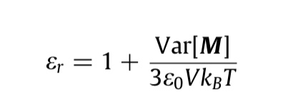
I am using the equation attached, eps_r = 1 + Var[M]/(3 eps_0 V kB T).
My units are all SI. The only possible problem I can think of is that I have somehow calculated the variance correctly. If anyone can see a problem with my method, I would be very grateful for a heads-up.
-
Here is example simulation output (for one time step):
-8.473356 1.553341 3.940367 # DIPOLE [BERRY PHASE][Debye]
-
I calculate a total dipole moment by summing the squares of these three components and then taking the square root. Then I convert to SI [F/m].
-
Here is where I may have made a mistake. I take that total dipole moment list/array and feed it into Python/numpy’s “var.”
np.var(totalMoment)
What I’m wondering is if this correctly represents the M term
It has been a long time since I did studies of dielectric properties of water models from computer simulations, so I had to look up some details from my PhD thesis.
Here are some brief points to consider:
- the value of the static dielectric constant will not be that of experimental water, but it a property of the water potential that you are using and can vary significantly with the choice of water potential
- how you can determine eps_r depends on the dielectric boundary conditions. you need to apply the correct fluctuation formula, or your results are going to be useless. many expressions in the literature are approximations and may not be valid for all simulation setups and may make assumptions not valid in your simulations
- you compute the total dipole moment by summing over the dipole moments of the individual water molecules, not over individual charges.
- you need very long trajectories to get converged values of the total dipole fluctuations (>> 1 ns).
- system size has a minor impact by comparison, it merely speeds up the validity of the approximation that ^2 = 0.0, not the convergence of <M^2>
for example, I computed a static dielectric constant for SPC water of 66 ± 3 from a 10ns simulation of 64 molecules and 67 ± 10 from a 2ns simulation of 512 water (this was in the late 1990s, so those trajectories took quite a bit of time and effort to accumulate…)
you can find some overviews of (older) results and how much they vary(!) in J.Chem.Phys. 109(12), 4927-4937 and Mol. Phys. 94(3), 577-579 both from 1998
the derivation of the correct fluctuation formula can be found in Mol.Phys. 50(4),841-858 and Chem. Phys. Lett. 95(4,5), 417-422 both from 1983, lots of useful information is also in the book “Theory of Simple Liquids”, by Hansen and McDonald
in general, i found that computing dielectric properties has many very subtle gotchas and complications that are not always obvious. it took me several months to properly understand what was going on and where i was making mistakes that needed to be corrected. so if you have worked on this only two weeks, you should not consider this a long time (unless you are, unlike me, a genius).
of course, I could also send you a copy of my PhD thesis which has my own results and a detailed summary of how to correctly compute those properties and discuss the results, but that is written in german, so it would be of limited use unless you are proficient enough in german.
axel.