Help with thermal conductivity

Dear Developers & Users,

I am a beginner in using Lammps. I am trying to calculate thermal conductivity of a silicon nanowire and for that I am trying to understand the Green Kubo method using the example of Solid Argon. I know this has been discussed several times in the mailing list, but unfortunately I have not been able to find out answers to the specific questions I have.

When I use the input script , I get a thermal conductivity of 0.288 W/mK. However, when I play around with the auto correlation parameters Nevery, Nrepeat,Nfreq, results start to become inconsistent. I have changed correlation length § from 1 to 2000 but, 200 gave me the best result of thermal conductivity. As I go away from the correlation length of 200, results get weird. The same is true for the ‘sample interval’ (s) parameter. I was wondering if there is a method for systematically selecting the auto-correlation parameters and also the simulation time. How do I check whether the HCAF has decayed to zero?

The script I use is the following

%%%%%%%%%%%%%%%

units real
variable T equal 70
variable V equal vol
variable dt equal 4.0
variable p equal 200 # correlation length
variable s equal 10 # sample interval
variable d equal $p*$s # dump interval

convert from LAMMPS real units to SI

variable kB equal 1.3806504e-23 # [J/K] Boltzmann
variable kCal2J equal 4186.0/6.02214e23
variable A2m equal 1.0e-10
variable fs2s equal 1.0e-15
variable convert equal {kCal2J}*{kCal2J}/{fs2s}/{A2m}

setup problem

dimension 3
boundary p p p
lattice fcc 5.376 orient x 1 0 0 orient y 0 1 0 orient z 0 0 1
region box block 0 4 0 4 0 4
create_box 1 box
create_atoms 1 box
mass 1 39.948

pair_style lj/cut 13.0
pair_coeff * * 0.2381 3.405

timestep ${dt}
thermo $d

equilibration and thermalization

velocity all create $T 102486 mom yes rot yes dist gaussian
fix NVT all nvt temp $T $T 10 drag 0.2
run 8000

reset_timestep 0

compute myKE all ke/atom
compute myPE all pe/atom
compute myStress all stress/atom virial

compute flux all heat/flux myKE myPE myStress

variable Jx equal c_flux[1]/vol
variable Jy equal c_flux[2]/vol
variable Jz equal c_flux[3]/vol

fix JJ all ave/correlate $s $p $d &
c_flux[1] c_flux[2] c_flux[3] type auto file J0Jt.dat ave running

variable scale equal {convert}/{kB}/$T/$T/$V*s*{dt}
variable k11 equal trap(f_JJ[3]){scale} variable k22 equal trap(f_JJ[4])*{scale}
variable k33 equal trap(f_JJ[5])
${scale}

thermo_style custom step temp v_Jx v_Jy v_Jz v_k11 v_k22 v_k33
run 100000
variable k equal (v_k11+v_k22+v_k33)/3.0

variable ndens equal count(all)/vol

print “average conductivity: $k[W/mK] @ T K, {ndens} /A^3”

%%%%%%%%%%%%%%%

Thanks

Sankha Mukherjee
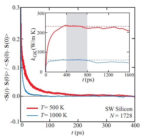
Sankha, you should be able to find a ‘plateau’ where the thermal conductivity doesn’t change much with sampling parameters. There are several papers out there on choosing parameters for GK. Here are some things you could check in the argon example:

the ACF should have enough points to be smooth and well-resolved.

the ACF should be long enough to decay to ~zero.
the ACF should be truncated not long after it has decayed.
the ACF should be averaged over many repetitions.

Tim

Hello Timothy,

Thanks for your reply. Would it work if instead of looking at the HCAF, I plot kappa as a function of time to see if the plot reaches a plateau? If it does, would it mean that HCAF has decayed to zero? I still do not know how to calculate the autocorrealtion function, so I am unable to check whether it is decaying to zero!! I have searched mailing list thoroughly and it seems everyone working on thermal conductivity in the community has figured out how to calculate the autocorrelation function, which I have not yet!

Thanks

Sankha

Actually you have calculated an ACF. Take a look at the G-K formula on the doc page for compute heat/flux, then look at the argon example line by line. You’ll see that the example computes heat flux, finds the ACF, and integrates ACF according to the G-K formula.

Tim

Hello Timothy,

I can not thank you more for all your help.

As per your advise, I have studied every command used in the script (copied in the first email). As I understand, the following is the part where the ACF is calculated.

fix JJ all ave/correlate $s $p $d &
c_flux[1] c_flux[2] c_flux[3] type auto file J0Jt.dat ave running

Now, do I get the ACF from the fix JJ? because to my understanding it is not in the J0Jt.dat file!

Correct me if I am wrong, since kappa is calculated by integrating (trap) f_JJ[3], f_JJ[4] and f_JJ[5], the ACF can be obtained from f_JJ[3], f_JJ[4] and f_JJ[5].

I have tried a lot to output f_JJ[3], f_JJ[4] and f_JJ[5] but did not have any luck. I have tried dump, thermo_style, nothing worked.

I do get the plateau in the thermal conductivity (as in the inset of the attached figure), but still do not know how to check whether ACF decays to zero!

May be I am asking too many questions, but I do not know how to get through this part…

Thanks

Sankha

Size effects in molecular dynamics thermal conductivitypredictions_Important.pdf (1.3 MB)

ACF.jpg

The bottom of the doc page explains the output columns of fix ave/correlate. You’re using the “auto” option with 3 input values, so there are 3 autocorrelations and some other info printed. This is printed to J0Jt.dat, since that’s what you asked for with the “file” option.

HTH,

Tim