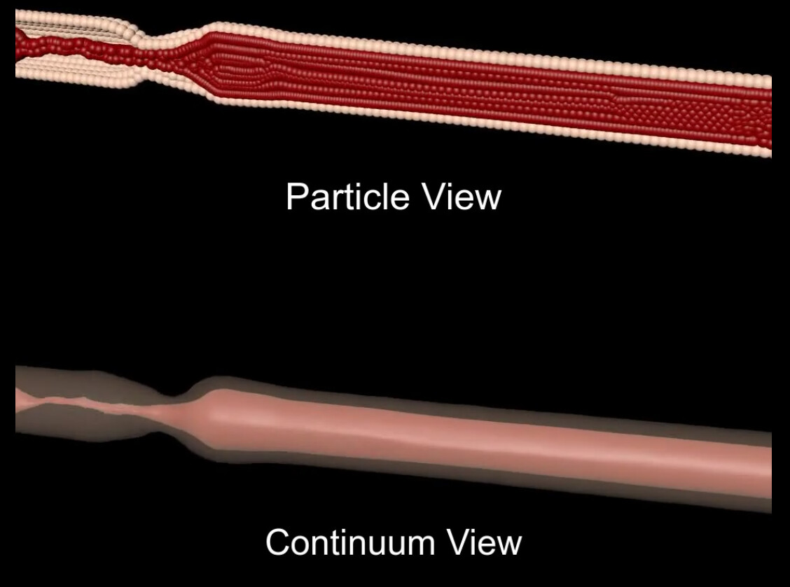
Usually, we visualize the LAMMPS simulation results in the particle (discrete) view. But here I am doing the SPH simulation and I want to have a continuum view of the results. I’ve known that in Paraview, it can be done by the SPH volume interpolation filter. How can it be obtained by OVITO?
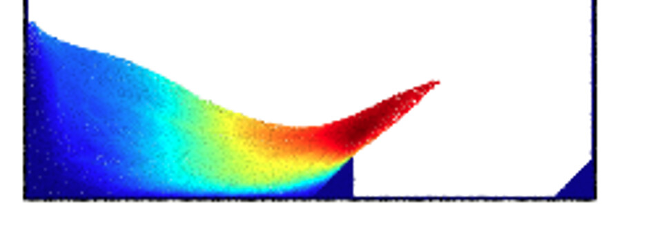
Below is an OVITO example from Alessio Alexiadis et al.'s research article (https://doi.org/10.1098/rsif.2020.1024) to help illustrate this question. Thanks in advance.
Hi, I see two possible workflows to create this kind of visualization.
You have the option to apply several instances of the Construct Surface Mesh modifier to your particle data and make use of its capability to take into account only a selection (subset) of particles. Construct surface mesh — OVITO User Manual 3.10.4 documentation
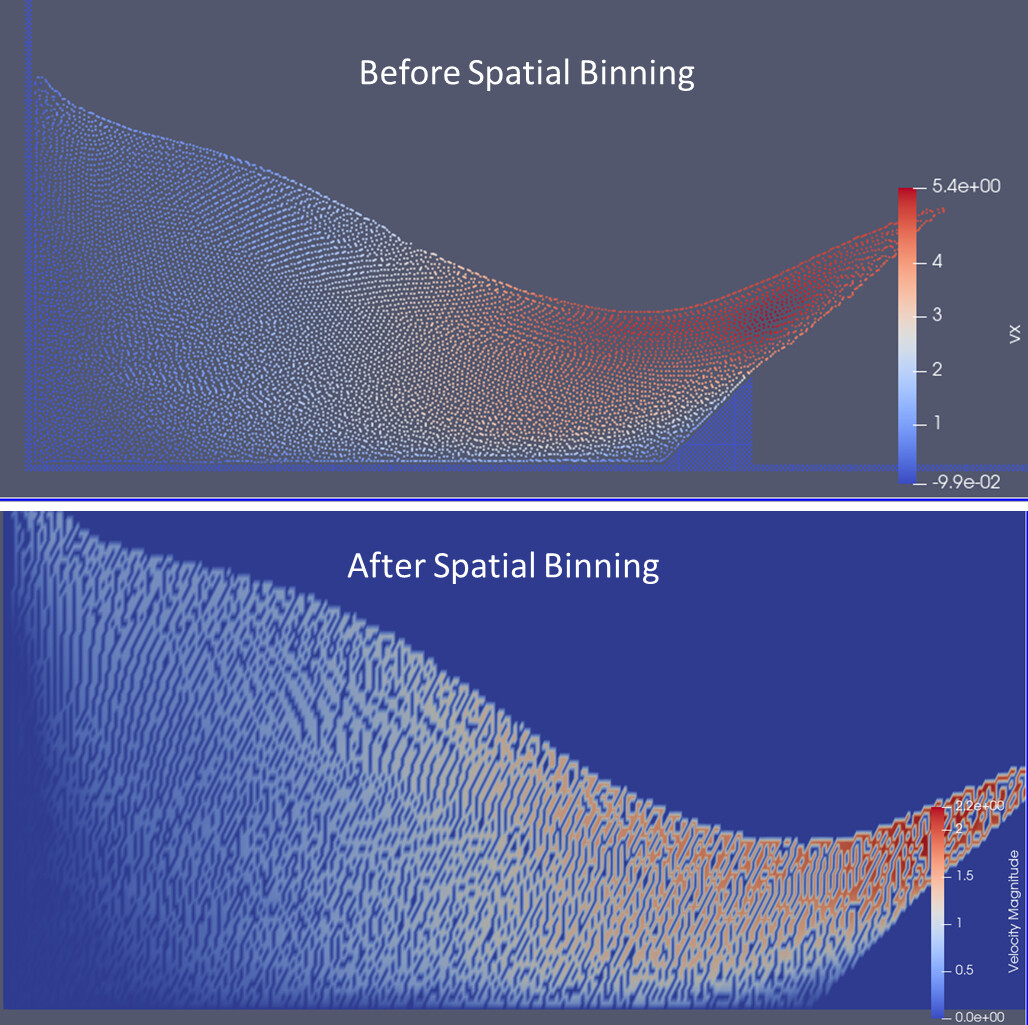
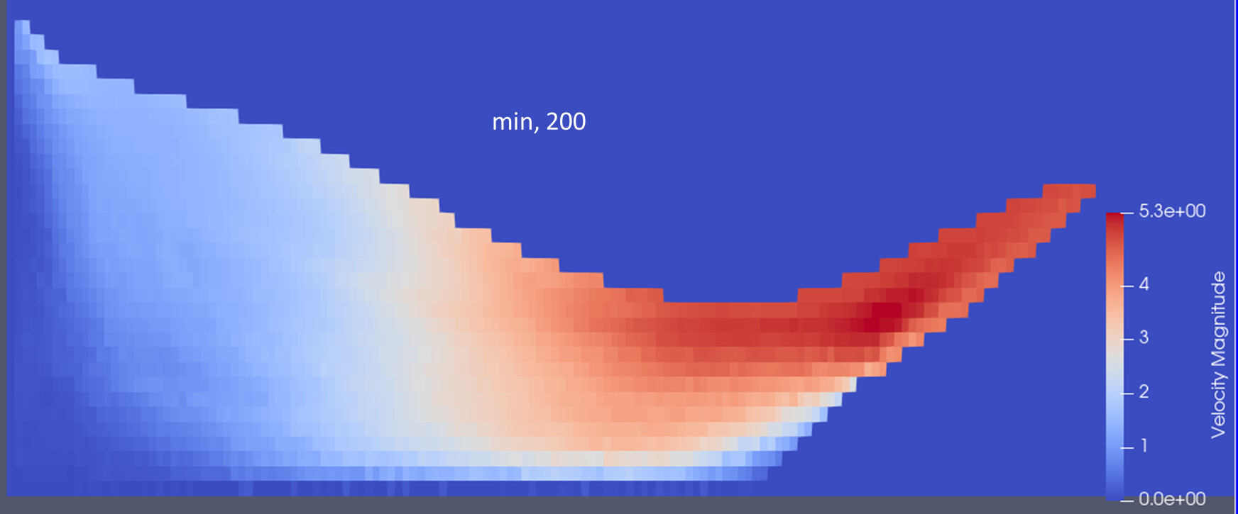
Hi @kalcher . I tried Spatial Binning to average the velocity as you advised. It doesn’t work for the water collapse case. The averaged velocities are very rough and change steeply.
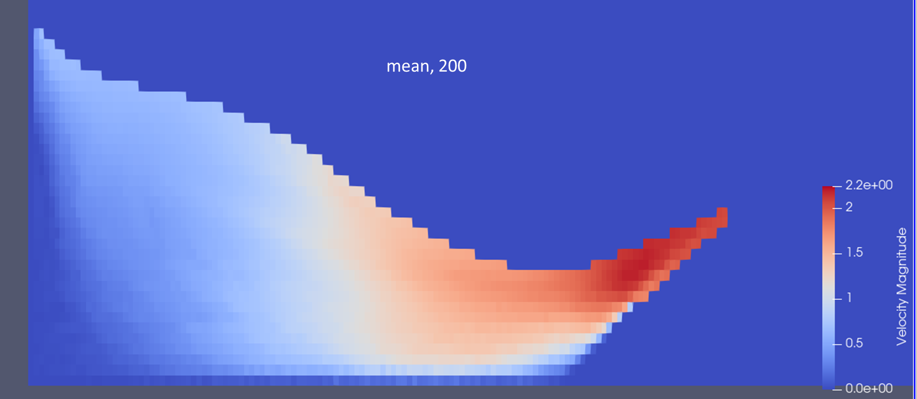
The min operation gave a good estimate out of surprise. In principle, it should yield lower values than mean.
This is not as expected. Could you send me the dump file used as input so I can replicate the analysis on my machine?
If you don’t want to share the data publicly you can also send me a DM here on matsci.
@utt Thank you for your interest. I tried to upload the dump file just now but was given “sorry, there was an error uploading that file”. Maybe I can alternatively email you the file if you are willing to provide the email address.
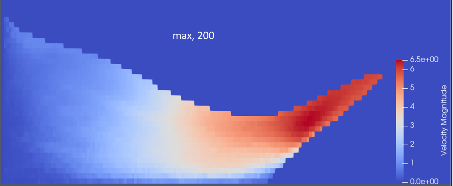
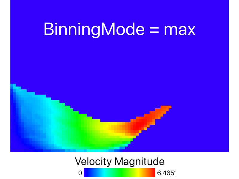
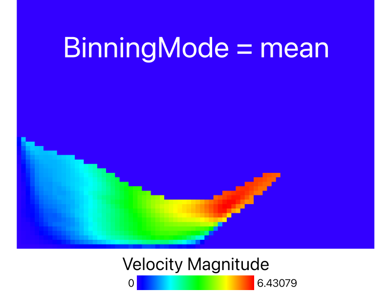
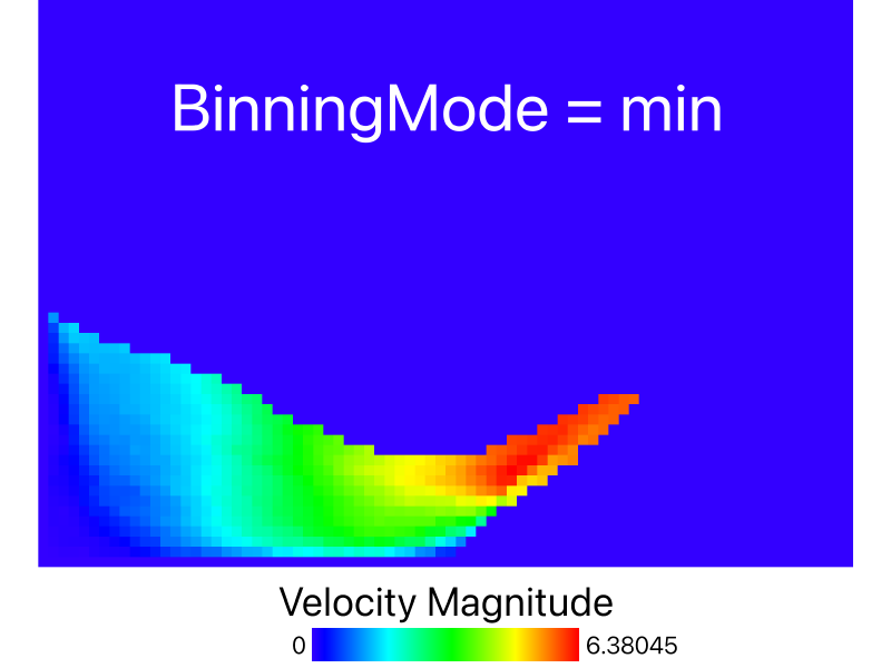
Thanks, I checked you file in OVITO and here the binning seems to work as intended. Using max as the operation give a value range from 0 to 6.46, using min gives a range from 0 to 6.38, and using mean results in values from 0 to 6.43. See the attached screenshot for reference.
Looks cool! Since I have no OVITO pro, I use the OVITO Python module to process data and use Paraview to visualize. Could you please provide the post-processing code for me (I mean for visualization because I am new to OVITO) to check quickly what is wrong?
Thank you utt. You provided SpatialBinningModifier code. What I wonder is how to visualize it in python. I guess it may need ColorCodingModifier? So I added it but only obtained a figure without binning.
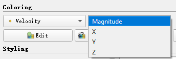
Finally, I realize where I went wrong. I specified the property as “Velocity” in SpatialBinningModifier originally and obtained underestimated velocity. Now I change “Velocity” to “Velocity Magnitude”, and the values look good in Paraview now.
The reason why I selected the property as “Velocity” was that the velocity in Paraview had X, Y, Z components and the magnitude. It is a vector and enables me to draw the arrow plot in Paraview.
Unfortunately, the values are wrongly estimated.