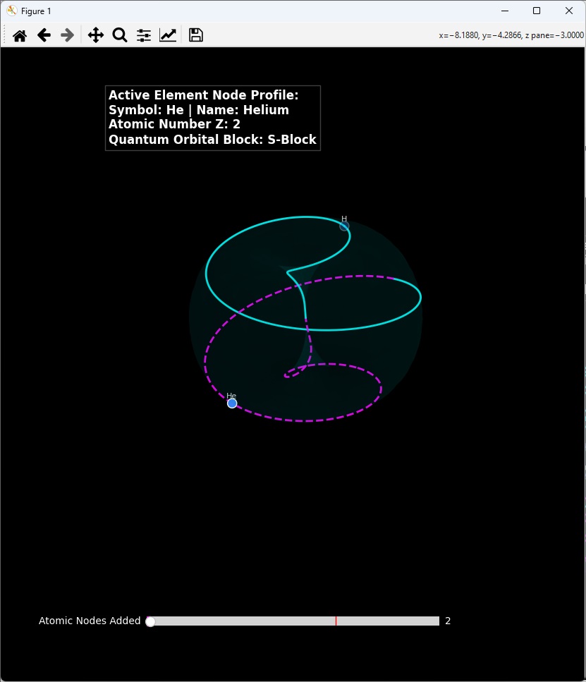
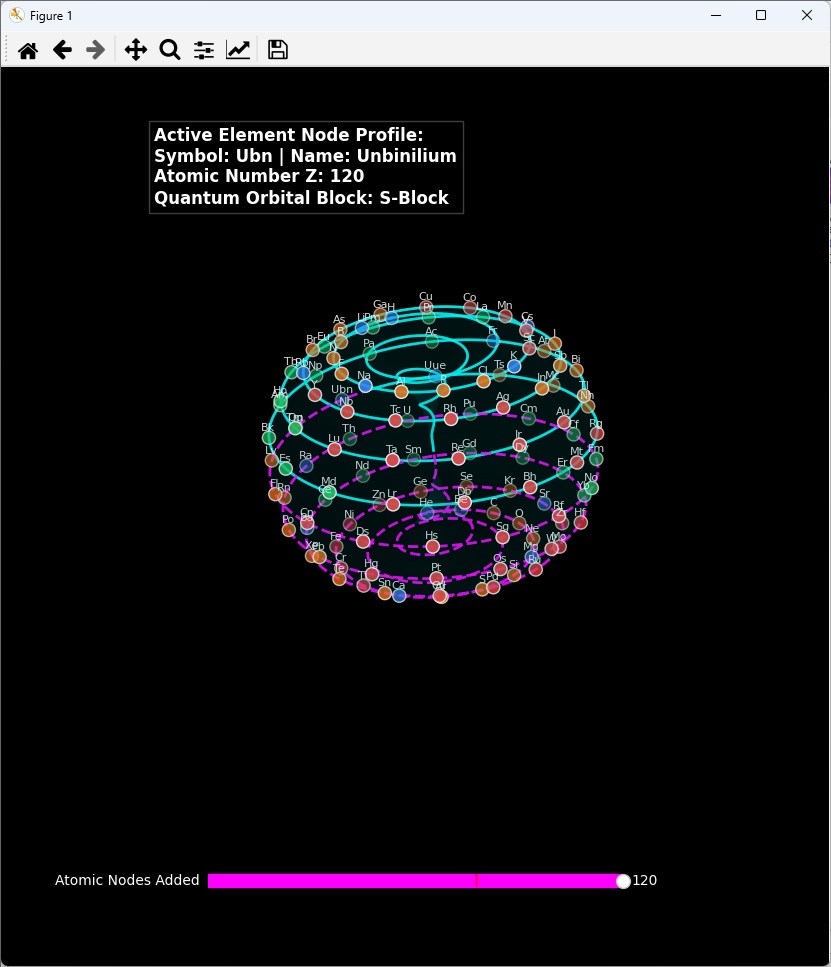
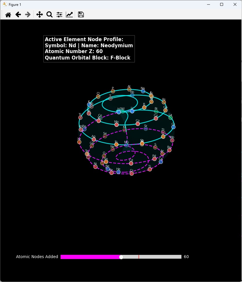
import numpy as np
import matplotlib.pyplot as plt
from matplotlib.animation import FuncAnimation
from matplotlib.widgets import Slider
— COSMETIC USER TOGGLE —
SHOW_SURFACE = True # Set to True to see the virtual surface skin, False to turn it off
-------------------------------------------------------------------------
1. FIXED QUANTUM SEQUENCE DATA MATRIX (1 TO 120) WITH STRINGS
-------------------------------------------------------------------------
Complete element lookup table for the corner display readout text box
element_names = {
1: (“Hydrogen”, “H”), 2: (“Helium”, “He”), 3: (“Lithium”, “Li”), 4: (“Beryllium”, “Be”),
5: (“Boron”, “B”), 6: (“Carbon”, “C”), 7: (“Nitrogen”, “N”), 8: (“Oxygen”, “O”),
9: (“Fluorine”, “F”), 10: (“Neon”, “Ne”), 11: (“Sodium”, “Na”), 12: (“Magnesium”, “Mg”),
13: (“Aluminium”, “Al”), 14: (“Silicon”, “Si”), 15: (“Phosphorus”, “P”), 16: (“Sulfur”, “S”),
17: (“Chlorine”, “Cl”), 18: (“Argon”, “Ar”), 19: (“Potassium”, “K”), 20: (“Calcium”, “Ca”),
21: (“Scandium”, “Sc”), 22: (“Titanium”, “Ti”), 23: (“Vanadium”, “V”), 24: (“Chromium”, “Cr”),
25: (“Manganese”, “Mn”), 26: (“Iron”, “Fe”), 27: (“Cobalt”, “Co”), 28: (“Nickel”, “Ni”),
29: (“Copper”, “Cu”), 30: (“Zinc”, “Zn”), 31: (“Gallium”, “Ga”), 32: (“Germanium”, “Ge”),
33: (“Arsenic”, “As”), 34: (“Selenium”, “Se”), 35: (“Bromine”, “Br”), 36: (“Krypton”, “Kr”),
37: (“Rubidium”, “Rb”), 38: (“Strontium”, “Sr”), 39: (“Yttrium”, “Y”), 40: (“Zirconium”, “Zr”),
41: (“Niobium”, “Nb”), 42: (“Molybdenum”, “Mo”), 43: (“Technetium”, “Tc”), 44: (“Ruthenium”, “Ru”),
45: (“Rhodium”, “Rh”), 46: (“Palladium”, “Pd”), 47: (“Silver”, “Ag”), 48: (“Cadmium”, “Cd”),
49: (“Indium”, “In”), 50: (“Tin”, “Sn”), 51: (“Antimony”, “Sb”), 52: (“Tellurium”, “Te”),
53: (“Iodine”, “I”), 54: (“Xenon”, “Xe”), 55: (“Caesium”, “Cs”), 56: (“Barium”, “Ba”),
57: (“Lanthanum”, “La”), 58: (“Cerium”, “Ce”), 59: (“Praseodymium”, “Pr”), 60: (“Neodymium”, “Nd”),
61: (“Promethium”, “Pm”), 62: (“Samarium”, “Sm”), 63: (“Europium”, “Eu”), 64: (“Gadolinium”, “Gd”),
65: (“Terbium”, “Tb”), 66: (“Dysprosium”, “Dy”), 67: (“Holmium”, “Ho”), 68: (“Erbium”, “Er”),
69: (“Thulium”, “Tm”), 70: (“Ytterbium”, “Yb”), 71: (“Lutetium”, “Lu”), 72: (“Hafnium”, “Hf”),
73: (“Tantalum”, “Ta”), 74: (“Tungsten”, “W”), 75: (“Rhenium”, “Re”), 76: (“Osmium”, “Os”),
77: (“Iridium”, “Ir”), 78: (“Platinum”, “Pt”), 79: (“Gold”, “Au”), 80: (“Mercury”, “Hg”),
81: (“Thallium”, “Tl”), 82: (“Lead”, “Pb”), 83: (“Bismuth”, “Bi”), 84: (“Polonium”, “Po”),
85: (“Astatine”, “At”), 86: (“Radon”, “Rn”), 87: (“Francium”, “Fr”), 88: (“Radium”, “Ra”),
89: (“Actinium”, “Ac”), 90: (“Thorium”, “Th”), 91: (“Protactinium”, “Pa”), 92: (“Uranium”, “U”),
93: (“Neptunium”, “Np”), 94: (“Plutonium”, “Pu”), 95: (“Americium”, “Am”), 96: (“Curium”, “Cm”),
97: (“Berkelium”, “Bk”), 98: (“Californium”, “Cf”), 99: (“Einsteinium”, “Es”), 100: (“Fermium”, “Fm”),
101: (“Mendelevium”, “Md”), 102: (“Nobelium”, “No”), 103: (“Lawrencium”, “Lr”), 104: (“Rutherfordium”, “Rf”),
105: (“Dubnium”, “Db”), 106: (“Seaborgium”, “Sg”), 107: (“Bohrium”, “Bh”), 108: (“Hassium”, “Hs”),
109: (“Meitnerium”, “Mt”), 110: (“Darmstadtium”, “Ds”), 111: (“Roentgenium”, “Rg”), 112: (“Copernium”, “Cn”),
113: (“Nihonium”, “Nh”), 114: (“Flerovium”, “Fl”), 115: (“Moscovium”, “Mc”), 116: (“Livermorium”, “Lv”),
117: (“Tennessine”, “Ts”), 118: (“Oganesson”, “Og”), 119: (“Ununennium”, “Uue”), 120: (“Unbinilium”, “Ubn”)
}
def get_block(z):
s_elements = [1, 2, 3, 4, 11, 12, 19, 20, 37, 38, 55, 56, 87, 88, 119, 120]
if z in s_elements:
return “s”
if z <= 10 or (13<=z<=18) or (31<=z<=36) or (49<=z<=54) or (81<=z<=86) or (113<=z<=118):
return “p”
if z <= 30 or (39<=z<=48) or (71<=z<=80) or (103<=z<=112):
return “d”
return “f”
R_TORUS = 2.5
raw_elements_list =
for z in range(1, 121):
hemisphere = “North” if z % 2 != 0 else “South”
name_str, sym_str = element_names.get(z, (f"Element {z}“, f"El{z}”))
raw_elements_list.append({
“z”: z,
“block”: get_block(z),
“hemisphere”: hemisphere,
“name”: name_str,
“symbol”: sym_str
})
-------------------------------------------------------------------------
2. MATCHING WINDOW SETUP & WEBELEMENTS COLOR MAPS
-------------------------------------------------------------------------
plt.style.use(‘dark_background’)
fig = plt.figure(figsize=(11, 9))
ax = fig.add_subplot(111, projection=‘3d’)
plt.subplots_adjust(bottom=0.25)
block_colors_map = {
“s”: “#3b82f6”, # Blue
“p”: “#f97316”, # Orange
“d”: “#ef4444”, # Red
“f”: “#22c55e” # Green
}
Backdrop wireframe matrix mesh
theta_mesh = np.linspace(0, 2np.pi, 60)
phi_mesh = np.linspace(0, 2np.pi, 60)
TM, PM = np.meshgrid(theta_mesh, phi_mesh)
X_mesh = (R_TORUS + R_TORUS * np.cos™) * np.cos(PM)
Y_mesh = (R_TORUS + R_TORUS * np.cos™) * np.sin(PM)
Z_mesh = R_TORUS * np.sin™
Renders wireframe or solid surface skin based on top toggle state configuration
if SHOW_SURFACE:
surface_object = ax.plot_surface(X_mesh, Y_mesh, Z_mesh, color=‘cyan’, alpha=0.06, shade=True)
else:
ax.plot_wireframe(X_mesh, Y_mesh, Z_mesh, color=‘cyan’, alpha=0.03, linewidth=0.5)
Initialize lines for the chronological segments of our single tracking thread
north_path_line, = ax.plot(, , , color=‘cyan’, linestyle=‘-’, linewidth=2.0, alpha=0.9, label=‘North (Solid)’)
south_path_line, = ax.plot(, , , color=‘magenta’, linestyle=‘–’, linewidth=2.0, alpha=0.9, label=‘South (Dashed)’)
inner_south_line, = ax.plot(, , , color=‘magenta’, linestyle=‘–’, linewidth=2.0, alpha=0.9)
inner_north_line, = ax.plot(, , , color=‘cyan’, linestyle=‘-’, linewidth=2.0, alpha=0.9)
scatter_nodes = ax.scatter(, , , s=90, edgecolors=‘white’, depthshade=True)
text objects to handle dashboard box readouts and node labels seamlessly
readout_text = ax.text2D(0.02, 0.95, “”, transform=ax.transAxes, color=‘white’,
fontsize=12, fontweight=‘bold’, bbox=dict(facecolor=‘black’, alpha=0.6, edgecolor=‘dimgray’))
text_labels_pool =
current_screw_angle = 0.0
-------------------------------------------------------------------------
3. PURE GEOMETRIC VORTEX ENGINE (DYNAMIC TIERS LENGTH STEPPING)
-------------------------------------------------------------------------
def get_pure_helical_coords(t_val, total_turns, screw_angle_deg):
theta = np.pi / 2 - (t_val * np.pi)
phi = (t_val * total_turns * np.pi) + np.radians(screw_angle_deg)
x = (R_TORUS + R_TORUS * np.cos(theta)) * np.cos(phi)
y = (R_TORUS + R_TORUS * np.cos(theta)) * np.sin(phi)
z = R_TORUS * np.sin(theta)
return x, y, z
def render_dynamic_toroid_spiral(screw_angle_deg, total_turns):
pts = 400
x1, y1, z1 = get_pure_helical_coords(np.linspace(0, 0.5, pts), total_turns, screw_angle_deg)
north_path_line.set_data(x1, y1)
north_path_line.set_3d_properties(z1)
x2, y2, z2 = get_pure_helical_coords(np.linspace(0.5, 1.0, pts), total_turns, screw_angle_deg)
south_path_line.set_data(x2, y2)
south_path_line.set_3d_properties(z2)
x3, y3, z3 = get_pure_helical_coords(np.linspace(1.0, 1.5, pts), total_turns, screw_angle_deg)
inner_south_line.set_data(x3, y3)
inner_south_line.set_3d_properties(z3)
x4, y4, z4 = get_pure_helical_coords(np.linspace(1.5, 2.0, pts), total_turns, screw_angle_deg)
inner_north_line.set_data(x4, y4)
inner_north_line.set_3d_properties(z4)
-------------------------------------------------------------------------
4. INTERACTIVE MASTER DRIVER LOOP
-------------------------------------------------------------------------
ax_slider = plt.axes([0.25, 0.08, 0.5, 0.03], facecolor=‘dimgray’)
node_slider = Slider(ax_slider, ‘Atomic Nodes Added’, 1, 120, valinit=78, valfmt=‘%d’, color=‘magenta’)
def render_frame(frame):
global current_screw_angle, text_labels_pool
current_screw_angle = (current_screw_angle + 1.2) % 360.0
max_active_nodes = int(node_slider.val)

# Clean previous node text objects to refresh efficiently without stacking ghosts
for txt in text_labels_pool:
    txt.remove()
text_labels_pool = []

total_turns = round(4.0 + (max_active_nodes / 120.0) * 12.0)
render_dynamic_toroid_spiral(current_screw_angle, total_turns)

# Update active dashboard box display metrics configuration dynamically
last_el = raw_elements_list[max_active_nodes - 1]
readout_text.set_text(
    f"Active Element Node Profile:\n"
    f"Symbol: {last_el['symbol']} | Name: {last_el['name']}\n"
    f"Atomic Number Z: {max_active_nodes}\n"
    f"Quantum Orbital Block: {last_el['block'].upper()}-Block"
)

x_nodes, y_nodes, z_nodes, color_list = [], [], [], []

for i in range(max_active_nodes):
    el = raw_elements_list[i]
    progress = i / max_active_nodes if max_active_nodes > 1 else 0.0

    if el["hemisphere"] == "North":
        path_t = progress * 0.5
    else:
        path_t = 1.0 - (progress * 0.5)

    xn, yn, zn = get_pure_helical_coords(path_t, total_turns, current_screw_angle)

    x_nodes.append(xn)
    y_nodes.append(yn)
    z_nodes.append(zn)
    color_list.append(block_colors_map[el["block"]])

    # Append fast text labels directly hovering above active coordinate nodes
    tl = ax.text(xn, yn, zn + 0.12, el["symbol"], color='white',
                 fontsize=8, ha='center', va='bottom', alpha=0.85)
    text_labels_pool.append(tl)

if x_nodes:
    scatter_nodes._offsets3d = (x_nodes, y_nodes, z_nodes)
    scatter_nodes.set_facecolors(color_list)
    scatter_nodes.set_edgecolors('white')
else:
    scatter_nodes._offsets3d = ([], [], [])

return north_path_line, south_path_line, inner_south_line, inner_north_line, scatter_nodes
ax.set_xlim(-5.5, 5.5)
ax.set_ylim(-5.5, 5.5)
ax.set_zlim(-3.0, 3.0)
ax.axis(‘off’)
ax.view_init(elev=25, azim=45)
ani = FuncAnimation(fig, render_frame, interval=20, blit=False, cache_frame_data=False)
plt.show()