[lammps-users] qeq/comb dynamics

[Martin_Seth_Curtis]

Hello,

I am trying to get a better grasp of the actual implementation of the dynamics in fix qeq/comb. I have seen it said that the charges are solved using damped dynamics and I have also seen it referred to as an extended Lagrangian method. If I understand correctly from the documentation, every Nevery timesteps the nuclear degrees of freedom are held fixed and the charges are propagated using damped dynamics until the convergence criteria is met and the charges are near there 0 K values, then the charges are fixed for another Nevery timesteps as the nuclei are time evolved. Effectively the charge dynamics are treated essentially independently from the nuclear dynamics.

If I understand the Rick, Stuart, and Berne paper, they don’t use damped dynamics for the charges, and the charge equations of motion are solved simultaneously to the system equations of motion, more akin to what I think of as an extended Lagrangian approach.

If I’m understanding the above two correctly, is there a reason that damped dynamics were used in fix qeq/comb instead of either just solving the unmodified equations of motion, or adding a thermostat as suggested in the Rick, et al. paper? And why not solve the equations of motion for all degrees of freedom simultaneously. I can imagine that if the charges need to be solved on a shorter timescale, one could use a multiple time scale integrator.

If I’m misunderstanding how fix qeq/comb works, can someone explain what I am getting wrong?

Thanks

Seth Martin (he/him/his)

PhD candidate

Dept. of Chemistry

The University of Kansas

[akohlmey]

There is a high-level discussion of several different charge equilibration methods in the documentation of the QEQ package fixes: https://docs.lammps.org/fix_qeq.html
Fix qeq/comb uses what the authors of the COMB and COMB3 potential chose. If you have questions about that choice, I suggest you study their publications and then contact the corresponding author(s) of those publications with your questions.

Axel.

[akohlmey]

… and my response about the why is the same, too: please look up and study the corresponding publications and contact the authors (of the papers and/or the fixes).

As maintainers of the LAMMPS code we don’t need to know why people make choices in their code, but whether their code gives the correct and intended results.

My suspicion is that the implementation of of an extended Lagrangian scheme is not as trivial as you seem to think it is. Please also keep in mind that the computational cost of computing/updating the electrostatic potential is similar to that of the force computation so that the total effort of an extended Lagrangian scheme will be determined by the choice of fictitious mass and how well the fictitious dynamics can be decoupled from the real dynamics (as those determine the maximum time step possible and the accuracy) while that of iterative methods depends on how many iterations are needed per qeq step (which is determined by the convergence/accuracy parameter).

My personal experience with Car-Parrinello DFT software has shown that an extended Lagrangian scheme is increasingly difficult to maintain for increasing system size (as this requires to increase the fictitious mass to avoid coupling to the atomic DOFs and thus reduces the accuracy) and that an iterative scheme can be quite competitive for larger systems, if not significantly faster if an effective extrapolation scheme is used to reduce the number of iterations required to reach convergence. Mind you in electronic structure MD the cost of computing/updating the electronic structure way outweighs the cost of computing the forces on atoms, so the situation is more extreme than in classical MD, but also the system sizes are way smaller. But this is just conjecture, for an authoritative answer you need to contact the people who implemented the schemes in LAMMPS and/or wrote the corresponding publications.

Axel.

[Martin_Seth_Curtis]

Thanks for the doc page Axel. Looking at that page, I have the same questions about qeq/dynamic as I do for qeq/comb. None of the methods described in the doc page seem to match the extended Lagrangian method as described in the Rick, Stuart, and Berne paper. If I understand the documentation for qeq/dynamic, it is essentially the same method as I described previously for qeq/comb.

Seth Martin (he/him/his)
PhD candidate
Dept. Of Chemistry
University of Kansas

[Ray_Shan2]

Hi Seth,

Actually fix qeq/comb uses the exact same extended Lagragian method proposed by Rick and Stuart but it only changes the charge’s equation of motion a bit (by adding a damping term to facilitate convergence).

Also, all qeq methods separate the electronic step (charge equilibration) and the ionic step (integrating atom’s equation of motion). This is the application of the Born Oppenheimer approximation that all DFT codes also use.

[akohlmey]

Ray,

in an extended Lagrangian scheme in the strict sense, you do not converge to the minimum (ground state in DFT), but you effectively treat the minimization of the “constraints” (i.e. the value of the charges) like additional, fictitious degrees of freedom (e.g. as harmonic potentials) and update them along the positions.
This requires to have the charges fully equilibrated only once at the beginning of a run, but then you will only do one iteration per MD step. For that to work, a fictitious mass has to be assigned to those fictitious degrees of freedom which crucially determines a) the possible maximum time step b) how much energy is exchanged between the two systems, which must be very little to make certain the equilibrated charges stay close to the optimum and are distributed in a symmetric gaussian distribution around that optimum, so that the error from not having fully optimized charges (mostly) cancels out. A larger mass usually leads to a better decoupling but at the same time, the mass must not be too large so that the optimum charge values are not “lagging behind” by too much. As mentioned in the previous email that becomes a problem for larger systems, because they allow a wider range of fluctuation frequencies and thus increase the coupling between the two systems.

In Car-Parrinello schemes, the electrons are treated as if they are orders of magnitude heavier to achieve that decoupling and that can become a problem for anything where there are fast changes in the electronic structure. Thus the time step is usually significantly shorter than for classical or Born-Oppenheimer MD. To improve the stability of such extended Lagrangian schemes one can apply a thermostat to those fictitious degrees of freedom which counteracts the energy transfer from the atomic system to the fictitious system but can also hide bad choices of parameters (similar to applying a thermostat for classical MD can hide non-conservation of energy due to choosing too large a timestep). In DFT the decoupling is related to the band gap and thus you will find very few studies of metals with Car-Parrinello schemes, as they are extremely difficult to manage and are dependent on a perfect balance between fictitious mass and thermostat parameters for the fictitious dynamics and the desired accuracy.

In contrast to that, Born-Oppenheimer approaches for the same DFT systems suffer from a (small) systematic friction due to using the electronic state from the previous state as the initial step. The amount of this friction (and thus non-conservation of energy) depends on how tightly the convergence is chosen and thus decides on the efficiency of this method. For a long time Car-Parrinello was considered more efficient (fewer evaluations of the electronic structure per absolute time, since achieving tight convergence with Born-Oppenheimer schemes would require a lot of iterations), but that changed when people applied extrapolation schemes like the ASPC method
( https://doi.org/10.1002/jcc.10385 ) which would then lead to a gaussian distribution of the initial guess around the converged minimum and then lead to similar error cancellation as with Car-Parrinello and thus no longer required as tight a convergence to accurate and energy conserving MD runs.

Axel.

[akohlmey]

based on my explanations from previous emails: are you certain, that your settings for COMB are calling the qeq/comb fix often enough and are converging tight enough?

apart from that, please note that it is usually more productive to provide a small and fast to run demo input that illustrates a problem so that people can look into where the cause of the issue is, rather than asking why not some other approach was used. As I tried to explain, in all of these schemes it is necessary that suitable settings are chosen to achieve good accuracy and energy conservation.

please also always report which LAMMPS version you are using and, if possible, try the latest available patch/development version to verify that you are not subject to a bug that has since been fixed.

Axel.

[Martin_Seth_Curtis]

Ray, the damped dynamics of qeq/comb and qeq/dynamic are still just finding charges that minimize the energy. This is something that bothers me about COMB3. It essentially does the same thing as strietz-mintmire and reaxff in terms of updating charges by finding the equilibrium charges, just with different minimization schemes. But COMB experiences an extremely rapid energy drain not seen in other reactive forcefield that use EEM methods for the charges.

Thank you for Axel for the explanation of the difference. To me, this distinction between a true extended Lagrangian approach like in Rick, er al. and the damped dynamics of qeq/dynamic and qeq/comb is not at all clear in the documentation.

Seth Martin (he/him/his)
PhD candidate
Dept. Of Chemistry
University of Kansas

[Martin_Seth_Curtis]

Sorry Axel, I maybe wasn’t precise enough in my original email. Really, the main issue I wanted to bring up is that while both fix qeq/comb and fix qeq/dynamic reference the Rick, Stuart, Berne paper, they don’t actually follow the methods outlined in that paper. I don’t think the documentation really explains what those fixes are doing. I suppose my reason for writing the email was to say I think the documentation should be more explicit about what is being done in those fixes, and to understand why they suggest that extended Lagrangian methods are implemented; none of the fixes on the fix qeq/point doc-page are extended Lagrangian methods, they are all some form of minimization.

In regards to the COMB energy drain, I didn’t mention it as a request for help trouble shooting. Based on previous mailing list discussions (https://sourceforge.net/p/lammps/mailman/message/36666819/) and discussions with a member of Susan Sinnott’s group this seems to just be a fact of COMB. I only mention it because I don’t know that I’ve ever been fully satisfied with the response I’ve seen that suggests the loss in energy is solely due to the charge dynamics, which as implemented are no more coupled to the nuclear dynamics than the matrix inversion method and therefore shouldn’t cause extremely rapid energy drain unless the settings are poorly chosen as you mention. But the responses that I’ve received from the Sinnott group is that COMB does have energy drain, and you need to use a thermostat to reach a steady state where the thermostat feeds energy in fast enough to counterbalance the energy drain.

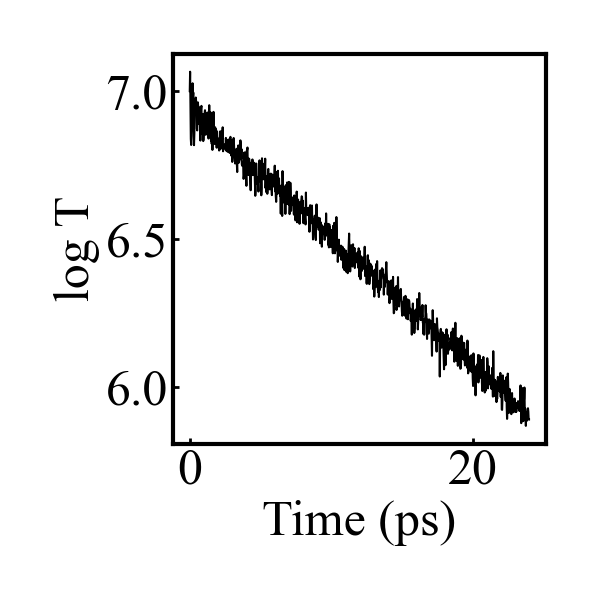
I’m finishing up my dissertation over the next couple months, but after I get settled in my new job in the fall I intend to take a deeper dive into the energy drain and related issues I’ve seen with COMB. Hopefully I can give a fuller picture then. As a quick example, though, here are the results for the bulk corundum simulation given below:

Even with a timestep of 0.05 fs, equilibrating the charges every timestep, and a tolerance of 0.00001 for the charge equilibration, there is an exponential decay in the Temperature (and total energy) once the thermostat is removed. Maybe I missed something in my simulation setup, but I don’t think there is anything in my simulation that would lead to this kind of exponential energy drain.

The figure is the log of the temperature after the thermostat is removed.

#simulation of corundum using COMB3

units metal

atom_style charge

dimension 3

boundary p p p

read_data data.small_corundum

variable comx equal vcm(all,x)

variable comy equal vcm(all,y)

variable comz equal vcm(all,z)

pair_style comb3 polar_off

pair_coeff * * ffield.comb3 O Al

neighbor 2.0 bin

neigh_modify every 1 delay 0 check yes

timestep 0.00005

thermo_style custom time temp press pe ke etotal v_comx v_comy v_comz

thermo 500

thermo_modify norm yes

fix 0 all qeq/comb 10 0.01

velocity all create 1043.0 42128 dist gaussian rot yes mom yes

minimize 1.0e-3 1.0e-3 100 1000

unfix 0

neigh_modify every 10 delay 0 check yes

fix 1 all qeq/comb 1 0.00001

fix 2 all nve

fix 3 all temp/berendsen 1043 1043 0.1

run 10000

reset_timestep 0

dump coords all custom 500 al_coord.lammpstrj id type q x y z

dump_modify coords sort id

unfix 3

velocity all zero linear

velocity all zero angular

run 500000

[Martin_Seth_Curtis]

I forgot my lammps version, which is 29 Oct 2020

Seth

[Ray_Shan2]

Hi Seth,

COMB’s qeq has a damping terms that drains energy so it is bound to lose energy conservation if charge equilibration is turned on. You could try first determine the equilibrium charge for the system, turn qeq/comb off, then run the same NVE test.

Ray

[Martin_Seth_Curtis]

Thank you for the response Ray. The reason I don’t think that the damping in the charge dynamics is a proper explanation of the energy drain is because the charge dynamics are separate from the dynamics of the rest of the system as implemented currently in fix qeq/comb. When the damped charge dynamics run, they essentially find the values of charges which minimize the energy. This is essentially the same thing that matrix inversion methods are doing, just using a different minimization algorithm. But none of the other variable charge force fields I have used have this exponential energy drain. I don’t see how the charge dynamics could be draining the energy from the nuclear degrees of freedom so rapidly when they are essentially uncoupled in the current implementation of fix qeq/comb as I understand it.

Seth