Melting simulation of Cu using EAM potential

Hi, I got a confussing problem when using the EAM potential for melting simulation. The potentials file I used is Cu_zhou.eam.alloy in the ./potentials directory. Below is my input file. The problem is when the temperature increase to 2050K, the system still have FCC structure. The version of lammps I used is lammps-5Jun19. I did the same simulation used the same version of lammps about one year ago, it work well, but today I can’t repeated the simulation results. Is anyone can help?

input file:
units metal
boundary p p p
atom_style atomic

lattice fcc 3.615

region box block 0 8 0 8 0 8

create_box 1 box
create_atoms 1 box

timestep 0.01

pair_style eam/alloy
pair_coeff * * Cu_zhou.eam.alloy Cu

neighbor 0.5 bin
neigh_modify every 5 delay 0 check yes

dump 1 all custom 1000 dump.cu_melt_position id x y z

thermo_style custom step temp pe ke press vol
thermo 1000

fix 1 all nvt temp 50 50 1 drag 0.2
run 20000
unfix 1

fix 1 all npt temp 50 2050 1 iso 0 0 10 drag 0.2
run 200000
unfix 1

fix 1 all nvt temp 2050 2050 1 drag 0.2
run 20000
unfix 1

Melting a solid need to overcome a finite energy barrier, so the simulation time required to observe the melting is somewhat random. And the result of MD simulations is usually not exactly reproducible due to floating-point arithmetic, especially when running in parallel and with packages like Intel or GPU. You may try running the last nvt simulation longer. Indeed I can get it melted with a somewhat more aggressive initialize method, though I don’t know if this is desired:

velocity all create 2050.0 4928459

fix 1 all npt temp 2050 2050 1 iso 0 0 10 drag 0.2
run 200000

Also there are lots of “dangerous builds” with your current neighbor settings, which means some of forces between atoms may be missed in the calculation. I would suggest increase the neighbor bin size or the frequently of neighbor list rebuilt (like neigh_modify every 1 delay 0 check yes). This may affect performance, so test it by yourself.

1 Like

Thank you very much for your reply. I have figured out the problem with your suggestion. After increased the timestep of first NVT simulation, the problem was solved. It seem that the running time of first NVT is too short to reach equilibrium, so the melting barrier increased artificially.

Hi @initialize,

This statement of yours:

is irrelevant. Floating-point arithmetic issues make some exact calculations hard to reproduce but are irrelevant concerning physics of large enough systems. Using the same potential and same input parameters should give the same general results in the case of large enough and long enough simulations.

@jw_Xie You conclusion is incorrect on the one hand and does not makes much sense on the other hand. No “melting barrier” can be increases or decreased by extending a simulation parameter. This is unscientific reasoning.

Here are a couple comments on your situation:

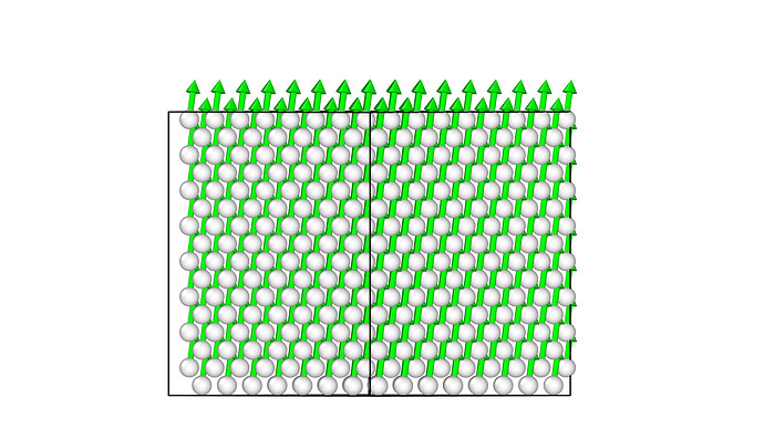
  • Your initial settings had no velocity and started with perfect crystalline position. What basically happened when taking you input as-is, is that you ended up with a flying ice cube at the end of your NVT run (see picture). You could see that because the potential energy does not change at all during the initial step of your simulation. This can still happen with NH thermostat when messing around with timestep values and is clearly unphysical. The rest of your simulation, from then on, was bogus.
  • “Increase the timestep” is vague. Did you increase the duration of the run? There is not much reason this could have mitigated the flying ice cube effect. Did you increase the timestep value? Then you must have a very good reason to do so because you are already using a very high value compared to what is typically used for solid metals. There are issues with increasing the timesteps regarding conserved quantities such as (pseudo)Hamiltonian energy. This is not a trivial thing to do and should be done with great caution. I would highly recommend sticking to the default 0.001 value in metal units and changing your Tdamp and Pdamp parameters accordingly.
  • Here your simulation parameters and setup are already odd and source of vigilance. But you should also update the LAMMPS version you’re using. The one you mention is nearly 4 years old which is very old in LAMMPS age. Many bugs have been corrected since then.
  • The correction to your issue was simply adding initial velocities to your atoms (velocity all create 50 <some random seed> followed by velocity all zero linear). However given the above comments, I would strongly recommend you to spend more time studying the MD literature and asking a double check on your MD setup and result from skilled advisor/supervisor/colleagues.

2 Likes

This is interesting and I can also observe this behavior. After some further tests I think that depend on the specific implementation, the Nose-Hoover thermostat may not work well with zero initial velocities. Indeed the problem is gone if I use the Intel variants (mpirun -n 8 lmp -sf intel -pk intel 0 omp 2 ...), presumably because it internally introduces some floating point noises on velocities (idk). This is probably why the author said it “worked well” before.

So the take-home message is probably that, to thermalize a system continuously from zero temperature (this is necessary sometimes), either assign some (small) random initial velocities or use another thermostat (like fix langevin).

My previous comments still applies in general (that is, for a process need to overcome a large energy barrier, it may or may not happen in a finite-length simulation depend on random factors), but it is unlikely a big problem in this specific case (2050K is way beyond the melting point of Cu and the melting barrier is generally smaller than crystallization).

1 Like

I think both the things you guys are saying about “reproducibility” are correct, but maybe you are saying different things.

I think @initialize is saying that picturing the melt event is somewhat “random”, being though more and more likely to occur depending on how much on the super-heated region you are (i.e., linked to the energy barrier thing mentioned). If the guy/girl had used in the beginning of the MD simulations two different velocity distributions corresponding to a T = 50K, it is very much possible that he wouldnt observe the melting literally at the same time step. And actually maybe 20000 timesteps at 2050K was not enough to observe the melting in the two different cases, being it then even possible to have a case in which one would have melted and the other not. But then this falls into what Germain may have meant with:

Using the same potential and same input parameters should give the same general results in the case of large enough and long enough simulations.

Concerning the influence the machine can have into reproducing precisely the same phase space trajectory in a context where the initial microstate and input script are precisely the same, I thiiiiink that (although I am not at all, not even remotely, the queen of informatics) it is possible to have divergences if the machines is different. I mean, it is possible that microstates given by the two machines at a same timestep is not the same. I am saying this because I remember at some point in the past I tried this for curiousity and the result was different despite me choosing the same amount of parallel processes. So then if running in different machines can lead to different phase space trajectories, it is in the roam of possibilities that he wont observe melting in one of them and observe in the other. So I agree with what @initialize said in the first comment. However I am unfortunately too ignorant in machines to be able to tell you what within the machine was making the microstate be different. And ofc however thermodynamic properties should be the same.

So maybe the guy/girl tried this in the past in a different machine and it worked. And maybe he managed to have enough time to make his system break free from this “flying xtal” effect (which I also found very interesting btw).

About this:

After some further tests I think that depend on the specific implementation, the Nose-Hoover thermostat may not work well with zero initial velocities.

Also, I think the main issue is maybe linked with the fact it is a crystal with the atoms sitting at perfect positions: if you had atoms out of order and things like that, I would guess that Nose-Hoover would not have problems in working with initial zero velocities (so this is not a problem for Nose-Hoover). I tried it for curiosity and my temperature adapted very quickly to the proper value together with the other properties.

1 Like

Btw, this NVT after the NPT is very akward… you may want to check that out since the final volume your system reaches after the NPT with (or even without) temperature ramp will not be the equilibrium volume corresponding to a T= 2050K and p = 0 bar for your system in the eyes of the force field.

Yes, this is a valid point. If the system is initially out of equilibrium, atoms will get non-zero velocities after a few steps, and the Nose-Hoover thermostat can work after that. The claim of “not work well with zero initial velocities” may be better worded as, the Nose-Hoover thermostat cannot heat up atoms with zero velocities by itself, unlike e.g. the Langevin thermostat which adds extra forces to atoms. This may be better demonstrated by using e.g.
pair_style zero, where the Nose-Hoover thermostat will have zero temperature at all time without a manual velocity create.

The Nosé-Hoover thermostat is designed to maintain a temperature in a way so that NVT ensemble like sampling can be achieved. In general, you want the impact of the thermostat to be minimal so the thermodynamic properties are minimally affected.

So starting with zero velocities is going against it’s design goals, and generally a waste of simulation time.

2 Likes

Yes, this is a valid point. If the system is initially out of equilibrium, atoms will get non-zero velocities after a few steps

Yes, thanks to the forces between the atoms :slight_smile:

If I have in mind correctly the precise expression according to which the Nose Hover acts on the momenta of the particles, I think that, if the atoms of that xtal were literally in the same precise relative distance of one another (without any tiny bit of difference) and therefore had a velocity with the same magnitude and direction as illustrated in Germain’s drawing, maybe the xtal would have been flying forever regardlessof the Nose Hover thermostat :"D

Anyways, interesting discussion

Hi @ceciliaalvares,

A couple of comments on your answers:

  • It might not have been clear but my figure is a simulation result from the input file provided by @jw_Xie. The arrows magnitude is arbitrary but their direction is the same.
  • I meant what I meant in my previous comments on numerical precision. Floating point arithmetic has nothing to do with the initial problem. The problem of diverging trajectories due either to floating arithmetic precision and chaotic behaviour is a different topic (you can read William Hoovers’ books on the topic, very interesting statistical mechanics textbooks).
  • Thermostats implementation or compilation are a different topic. There can be different way of initializing the thermostat fictious particles depending on the implementations. That, I do not know. However, such differences should not affect reproducibility of expected physical behaviour with reasonable simulation setup. Bypassing bogus setup by using a different implementation is a bad idea IMHO.

Hi @Germain,

I understand that the magnitudes of velocities were not precisely the same. If they were, I think (although not sure) you would not have been able to get out of the flying xtal state using the Nose-Hoover thermostat. I understood that your drawing is qualitative and it was just to illustrate your point.

I am not trying to say that there are not other problems with the initial input script that @jw_Xie used. But if @jw_Xie ran precisely the same simulation (with the same input file) 1 year ago versus now, I suppose that, given how strict you are suggesting that the calculations are, he would have gotten the same result, regardless of it being bogus results or not. Yet, in one case he managed to melt it and in another he didnt. This is so regardless of the “create velocity” and being stuck for a while in a flying xtal, since he didnt initialize velocities in neither of the two cases.

So, despite understanding that he should have initialized the system with velocity in order to do things correctly, I disagree that this is the reason why he got different results in the past vs now.

Now just one last comment on my side so that we dont start a conference on the topic:

Be it due to floating points (and its propagation) or not, I have noticed that a calculation starting with a same input can lead to different microstates at a same precise time instant when I run the simulation at different machines - and I am talking of positions of atoms that are different by more than a 1E-10 value or whatever (see the example below). Of course the structure of my system is the same as so are the other macroscopic properties (otherwise we would all be lost). And of course that, in the case of phase transition, if the force field predicts an underlying melting temperature of X K for the system, the simuation in both machines would be able to picture the event with a same probability rate when I am at a same given temperature (which may however happen at different timesteps if indeed there is a difference in phase space trajectory or if the trajectories are meant to be the same but different by a given delta_value, I dont know). So, putting the other issues in the guy’s script aside and aiming to explain solely the difference in results from when he ran the simulation 1 year back versus now, I think @initialize may have a point when he talks about it “not being exactly reproducible” in a context where someone is trying to depict something such as a phase transition.

eg:
in two simulations done with a same precise input file, each made in a different machine (although I realize now that the amount of parallel processes is not the same, in case it adds up to something), I have, at time step 1m:
atom 238 at (0.865873, 5.3675667, 7.1528388) in one machine and at (0.61354, 5.60639, 6.97725) in the other machine.
This subject starts to be a bit too long and clearly off-topic but allow me to clarify a last time:

  • The magnitude were the same, only the vectors length on the picture is arbitrary. Velocity vectors length means nothing in a 3d space without a scale.
  • Those were simulation results from the input script provided.
  • This was a flying ice cube obtained using the NH thermostat. I did not deny that.

Now:

If OP did the exactly same thing and got different result, then something was different either on software or hardware and it was not exactly the same. In both case without the info, I discard this statement as not relevant to the problem at hand and the question they asked. They have a flying ice cube due to bad setup today. If they had “good results” last year, their setup was still wrong and the said “good results” have now to be explained.

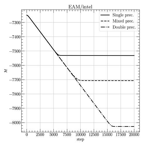
For example, after doing some more tests after @initialize idea to use the intel package I discovered that the reason it worked is because the default mode of the intel package is mixed mode where forces are calculated in single precision but stored in double precision. Using the double mode gives once again a flying ice cube while single precision also makes the problem go away. I attach here a picture of the different values the conserve quantity converge to for illustration. So there is floating point precision at hand but because the default introduces noise. Now this was assuming OP used the intel package in the past which is not stated, and this is clearly a very wrong workaround.

Some additional comments of my own :slight_smile:

Running a simulation on different numbers of processes is all but certain to give computationally different results. Each processor will have a different number of atoms, and therefore definitely a different order over which forces are accumulated, as well as a different partitioning of forces between processors at boundaries.

The Nose-Hoover thermostat is known to have poor ergodicity for ideal harmonic oscillators, and a perfect starting lattice is about as strongly harmonic a multibody system as you can get. You can see this qualitatively in the equation of motion: \dot{\mathbf{p}}= \mathbf{F}-\alpha \mathbf{p}. If all particles have parallel momenta, the thermostat simply rescales them and leaves them parallel. There’s nothing in the thermostat to change that and thus transfer energy into the higher-frequency modes, as compared to a Langevin or Andersen thermostat.

Having said that, the Nose-Hoover thermostat will still do a reasonable job of sampling a canonical ensemble if started from a reasonable starting point. It at least “breaks early”, in that you should be able to diagnose non-ergodicity early on. Some purists (not me!) would restrict “flying ice cube” to situations where the thermostat actively siphons energy from high-frequency into center-of-mass modes (as opposed to starting from 0K and simply not being able to excite HF modes from a poor start), since such a situation would show up later in a situation and taint a long-running trajectory.

In particular, whenever “flying ice cube effect” is mentioned, I automatically think of this paper: https://pubs.acs.org/doi/10.1021/acs.jctc.8b00446 which has made me intensely allergic to the Berendsen thermostat.

2 Likes

You can see this qualitatively in the equation of motion: ˙p=F−αp. If all particles have parallel momenta, the thermostat simply rescales them and leaves them parallel.

Yeah, this is what I had in mind when I said that if the velocities in a (qualitative) scenario as Germain depicted had exactly the same magnitude, I dont think the Nose-Hoover thermostat would ever be able to set it free from being a flying xtal.

Running a simulation on different numbers of processes is all but certain to give computationally different results.

Thanks for the clarification! :slight_smile:

It is just that apparently when the explanation comes from you, you get claps and roses throw in your direction, but when I say the same thing mentioning a figure to assist me in making my point, I get a full lecture about how the green arrows in the figure do not have quantitative meaning and also how you need to have a scale to be able to infer about vector’s magnitudes.

But no feelings hurt, let’s just move on :")

Please, just a last edit for my own peace of mind and then I promise I stop talking about this:

I was insisting about the magnitudes of the velocity being exactly the same because in a scenario where the velocities do not have the same magnitude and are simply parallel to one another, eventually the particles would also have a different positioning relative to one another. And if that happened, the force each of them experience would start to be different. Depending on the symmetry of force-field, this would start causing a different direction of individual momenta of the particles, breaking the flying xtal state. This was what I had in my mind when I stated that if both, initial direction and velocity magnitudes were the same, I believed the system would never break free from being a flying xtal.

1 Like

I should have closed this discussion a couple of days ago and suggested to create a new topic in “Science Talk” about what can be reproduced in simulations and under which circumstances and what not. Sorry for not paying enough attention. Will do so now.