Dear all users.
Hello and thank you for your kind answer and I have a question today.
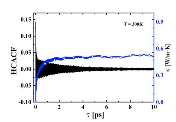
I use the Green-Kubo relation to calculate the thermal conductivity of Si/Ge materials.
The equilibration time is long enough (5x10^8, i.e, 50ns, timestep=0.04fs,) and the calculation time is 5x10^7 (i.e, 5ns, 0.04fs).
Not all specimens, but some results show the values of K_x or K_y are minus.
I attached the part of log.lammps. Was it wrong or is it common happening??
How can I deal with it?
Always, Thank you !
Soon-sung
Memory usage per processor = 5.30811 Mbytes
Step Temp v_Jx v_Jy v_Jz v_k11 v_k22 v_k33
44000000 314.7088 0.013884877 0.0013452806 -0.025071005 0.002986224 0.25441179 47.391615
45000000 306.65114 -0.017932204 0.016438403 0.022610574 0.0065858527 0.45452781 44.620341
46000000 308.55702 0.025219713 -0.0091908937 0.00028807707 -0.086013941 0.56157795 42.904199
47000000 307.11377 0.01324978 -0.0043413537 0.0056092352 -0.12102137 0.60298632 42.467715
48000000 310.15806 0.021765644 -0.0069727233 -0.0033735036 -0.14967663 0.59212901 46.366065
49000000 310.43336 0.011451546 0.0048310751 -0.0062498359 -0.16777871 0.63587463 47.680082
50000000 312.75731 0.023684767 0.0098494801 -0.0074646856 -0.19609388 0.59847542 47.869611
Total # of neighbors = 28756
Ave neighs/atom = 27.3867
Neighbor list builds = 77082
Dangerous builds = 0
Thermal conductivity : -0.196093882232808 [W/mK] @ 298.13 K
Thermal conductivity : 0.598475424509413 [W/mK] @ 298.13 K
Thermal conductivity : 47.8696111100201 [W/mK] @ 298.13 K
average conductivity: 16.0906642174322[W/mK] @ 298.13 K, 0.0423966362636883 /A^3