To the many users who have implemented a coexistence/two-phase method, what is the preferred implementation in LAMMPS? I’m new to MD and have scripts for two implementations I’ve identified by reading the relevant threads on here, but I am not satisfied with how I recombine the solid and liquid phases. In one implementation, I use ‘read_data’ to read in separate solid and liquid data files and combine them before equilibrating in NPH. In the other, I do it all in one input script, defining the top ~half of atoms as liquid and the bottom as solid. Is there a way to group atoms other than by region and other than by using ‘read_data’? How do I know how big my final simulation box needs to be? I’ve included my code below. Thanks in advance.
Luke
Implementation 1:
LIQUID
clear
units metal
dimension 3
boundary p p p
atom_style atomic
atom_modify map array

variable timeStep equal 0.001			# one femtosecond time step
timestep ${timeStep}

lattice fcc 3.615 origin 0.0 0.0 0.0 orient x 1 0 0 orient y 0 1 0 orient z 0 0 1
region box block 0 5 0 5 5 10
create_box 1 box
create_atoms 1 box

pair_style eam/alloy
pair_coeff * * Cu01.eam.alloy Cu

reset_timestep 0

velocity all create 100 654321 mom yes rot no dist gaussian
fix equilibrate all npt temp 100 1800 1 z 1 1 1 drag 0.2		# equilibrate to well above melting pt
thermo 1000
thermo_style custom step temp vol press
run 500000										# run simulation for 0.5 nanoseconds
write_data liquid.dat
unfix equilibrate

clear
SOLID
clear
units metal
dimension 3
boundary p p p
atom_style atomic
atom_modify map array

variable timeStep equal 0.001			# one femtosecond time step
timestep ${timeStep}

lattice fcc 3.615 origin 0.0 0.0 0.0 orient x 1 0 0 orient y 0 1 0 orient z 0 0 1
region box block 0 5 0 5 0 5
create_box 1 box
create_atoms 1 box

pair_style eam/alloy
pair_coeff * * Cu01.eam.alloy Cu

reset_timestep 0

velocity all create 100 654321 mom yes rot no dist gaussian
fix equilibrate all npt temp 100 100 1 iso 1 1 1 drag 0.2		# equilibrate to well below melting pt
thermo 1000
thermo_style custom step temp vol press
run 500000
write_data liquid.dat
unfix equilibrate

clear
COMBINED
clear
units metal
dimension 3
boundary p p p
atom_style atomic
atom_modify map array

variable timeStep equal 0.001
variable x1 equal "step"
variable x2 equal "vol"
variable x3 equal "temp"

timestep ${timeStep}

region box block 0 5 0 5 0 15
read_data solid.dat group solid
read_data liquid.dat add append shift 0 0 5 group liquid
pair_style eam/alloy
pair_coeff * * Cu01.eam.alloy Cu

reset_timestep 0

fix equilibrate all nph x 1.0 1.0 0.5 y 2.0 2.0 0.5 z 3.0 3.0 0.5
fix data_equilibration all print 100 "${x1} ${x2} ${x3}" file coexistence1.dat screen no
thermo 1000
thermo_style custom step temp vol press
run 10000000
unfix equilibrate
unifx data_equilibration
Implementation 2:
clear
units metal						# Angstroms, picoseconds, eV, Kelvin, bars
dimension 3
boundary p p p
atom_style atomic
atom_modify map array

variable tempLiquid equal 1800		# liquid temperature
variable tempSolid equal 300			# solid temperature
variable tempMelt equal 1400			# melting temperature estimate
variable timeStep equal 0.001			# one femtosecond time step
variable runTime equal 500000                # default run time of 0.5 ns

variable tempDamp equal "v_timeStep*100"		# temperature relaxed every 100 time steps
variable pressureDamp equal "v_timeStep*1000"	# pressure relaxed every 1000 time steps

variable x1 equal "step"
variable x2 equal "vol"
variable x3 equal "temp"

timestep ${timeStep}

lattice fcc 3.615 origin 0.0 0.0 0.0 orient x 1 0 0 orient y 0 1 0 orient z 0 0 1
region box block 0 5 0 5 0 5 units lattice							# simulation cell
region box2 block 0 5 0 5 5 10 units lattice
create_box 1 box
create_atoms 1 box

region lower block 0 5 0 5 0 2
region upper block 0 5 0 5 3 5
group lower region lower		# 'lower' refers to atoms in bottom of simulation box
group upper region upper		# 'upper' refers to atoms in top of simulation box

pair_style eam/alloy					# potential type
pair_coeff * * Cu01.eam.alloy Cu			# file name of EAM potential for Copper

reset_timestep 0

velocity all create ${tempSolid} 238232 mom yes dist gaussian
fix equilibrate upper nvt temp ${tempSolid} ${tempLiquid} ${tempDamp} drag 0.2
thermo 1000
thermo_style custom step temp vol press
run ${runTime}
unfix equilibrate

reset_timestep 0

fix equilibrate upper npt temp ${tempLiquid} ${tempMelt} ${tempDamp} z 1 1 ${pressureDamp} drag 0.2
thermo 1000
thermo_style custom step temp vol press
run ${runTime}
unfix equilibrate

reset_timestep 0

fix equilibrate all nph x 1.0 1.0 0.5 y 2.0 2.0 0.5 z 3.0 3.0 0.5
fix data_equilibration all print 100 "${x1} ${x2} ${x3}" file coexistence.dat screen no
thermo 1000
thermo_style custom step temp vol press
run 1000000                                                                                      # run for 10 ns
unfix equilibrate
unfix data_equilibration
If you are new to MD, you should be attempting a coexistence simulation as your first project. This is an advanced topic and you should be building your skills gradually with simpler projects first. In this case the simulation of individual solid and liquid bulk systems of your material of interest and comparing them to published results would be a natural choice. Have you discussed your approach with your adviser/tutor? They should have suggested the same thing.
Please explain what is the cause of your dissatisfaction.
Please see the documentation for the group command for other options. But I don’t quite see the need, so please explain what exactly you think you need and why.
You should be able to tell from making studies of the individual bulk systems in either liquid or solid state at the expected melting temperature. For metals, there should not be much of a difference that it would make much of a difference. Once you have a restart of the system with the two phases properly equilibrated, you can always start an exploratory simulation with (anisotropic) fix npt to see what the system itself equilibrates to.
I personally strongly favor this approach as it is more effective and has fewer sources of errors. Combining two separate systems causes a severe disruption because you are putting systems in contact that were proviously relaxed to a different geometry. Thus you need to leave some extra space to avoid overlaps (and then equilibrate it away) or find a way to remove the overlaps and then you would still need to content with having to dissipate shockwaves from the combining.
Thanks, Dr. Kohlmeyer. Yeah I seemed to have better luck with the second implementation, which was also recommended by my advisor. The need to leave extra space upon recombining the systems, as you mentioned, is where my dissatisfaction lies. Namely, how much? Is there an optimal value? If I don’t leave enough, the temperature increases drastically and atoms are lost in the simulation.
In regards to the ‘group’ command, I’d like to know how to put exactly one half of the atoms in the simulation into one group (e.g. the liquid group) and the other half into the other (solid group). If I group by region, defining one half of the simulation box as ‘liquid’ and the other as ‘solid’, there are atoms on the boundary of the two regions and thus those atoms belong to both groups (at least I think that’s what’s going on). If I remember correctly, for 864 atoms, the ‘liquid’ group contains 500 atoms and the ‘solid’ group contains ‘432’ (not sure why they’re unequal). I don’t know how much this kind of discrepancy matters in a coexistence method (maybe matters less for greater N), but I’d like to have each phase be the same size.
I believe I’m also missing a ‘fix’ for the solid group in the second implementation. If I want to fix the z-coordinates of a group of atoms, I can use ‘fix move’, correct? Something like this:
That is why I recommend against it. It just adds complications. The shockwave formation is less obvious and will not result in a crashing simulation, but will still taint your results. Thus the second option is the way to go.
That is a consequence of you you define your box/regions and lattice geometry. If you have a lattice that coincides with the box/region boundaries, you have ambiguities about where the atoms “belong”. This is easily avoided by either not selecting box/region boundaries to be exactly on the lattice points (e.g. region box block -0.1 4.9 -0.1 4.9 -0.1 4.9 instead of region box block 0 5 0 5 0 5) or by shifting the origin of the lattice definition (using origin 0.1 0.1 0.1 instead of origin 0.0 0.0 0.0). Either of the two options lifts the ambiguity and the issue should be avoided.
Two comments on that.
Please do not use the term “fix” in this context. In LAMMPS the term “fix” has a specific meaning because of the fix commands. It also does not really describe what you are after. A more correct term would be “immobilize”.
There are different ways to immobilize atoms. I think it would be a mistake to apply them here. Fix move is not correct in this setup, since it will time integrate atoms twice and that creates bogus results. LAMMPS warns about that. You can operate on the two sections of your input simply by applying fix nvt only to one part of the system and alternate a few times between the two until each part has equilibrated to the desired state and also the interface sufficiently relaxed. For the production run, you would apply the same time integration fix to the entire system since you need to let the phase boundary evolve.
A few more questions concerning my latest input script (below).
For a damping parameter of 0.5, that is to say that the temp/pressure is relaxed over half of a time unit, correct (for metal units, half of a picosecond)? For an equilibration performed at constant temperature, will a smaller pressure damping parameter lead to longer equilibration times?
If I want to allow atoms to relax in the ‘z’ direction and specify ‘z 1.0 1.0 0.1’ for an equilibration, do the ‘x’ and ‘y’ dimensions take default Pstart, Pstop, and Pdamp values?
clear
units metal						# Angstroms, picoseconds, eV, Kelvin, bars
dimension 3						# three dimensions
boundary p p p					# periodic boundaries
atom_style atomic
atom_modify map array

variable tempLiquid equal 1800		# liquid temperature
variable tempSolid equal 100			# solid temperature
variable tempMelt equal 1400			# melting temperature estimate
variable timeStep equal 0.001		# one femtosecond time step
variable time_eq equal 500000

variable tempDamp equal "v_timeStep*100"		# temperature relaxed every 100 femtoseconds
variable pressureDamp equal "v_timeStep*1000"	# pressure relaxed every 1000 femtoseconds

variable x1 equal "step"
variable x2 equal "vol"
variable x3 equal "temp"

timestep ${timeStep}		# create 'timestep' variable to reset later on

lattice fcc 3.615 origin 0.1 0.1 0.1 orient x 1 0 0 orient y 0 1 0 orient z 0 0 1	# 3.615 Angstroms between atoms
region box block 0 14 0 14 0 14 units lattice							# simulation cell
create_box 1 box
create_atoms 1 box

region lower block 0 14 0 14 0 7
region upper block 0 14 0 14 7 14
group lower region lower		# 'lower' refers to atoms in bottom of simulation box
group upper region upper	# 'upper' refers to atoms in top of simulation box

pair_style eam/alloy					# potential type
pair_coeff * * Cu01.eam.alloy Cu			# file name of EAM potential for Copper

reset_timestep 0

velocity all create ${tempMelt} 238232 mom yes dist gaussian
fix equilMelt all npt temp ${tempMelt} ${tempMelt} ${tempDamp} iso 1 1 ${pressureDamp}
thermo 1000
thermo_style custom step temp vol press
run ${time_eq}
unfix equilMelt

reset_timestep 0

fix equilLiquid upper npt temp ${tempMelt} ${tempLiquid} ${tempDamp} z 1 1 ${pressureDamp}
thermo 1000
thermo_style custom step temp vol press
run ${time_eq}
unfix equilLiquid

reset_timestep 0

fix equilLiquid2 upper npt temp ${tempLiquid} ${tempMelt} ${tempDamp} z 1 1 ${pressureDamp}
thermo 1000
thermo_style custom step temp vol press
run ${time_eq}
unfix equilLiquid2

reset_timestep 0

fix equilAll all nve
#fix equilAll all nph x 1.0 1.0 0.5 y 1.0 1.0 0.5 z 1.0 1.0 0.5
fix data_equilibration all print 1000 "${x1} ${x2} ${x3}" file coexistence_Preformatted textNVE_20_nanoseconds.dat screen no
thermo 1000
thermo_style custom step temp vol press
run 20000000
unfix equilAll
unfix data_equilibration
Only if the system is in equilibrium. To understand the process you have to understand the “mechanics” of a Nose-Hoover thermostat or barostat. It is a bit easier to understand for the thermostat. Basically, you have a set of coupled harmonic oscillators that are coupled to the force of the atoms. The damping parameter sets the fictitious mass(es) of these oscillators and thus determines their characteristic frequency, so you want to choose a damping time in such a way that the fictitious oscillators weakly couples to the atoms. Thus you try to choose the frequency so that it is in the vicinity, but not too close to some peak in the infrared spectrum of the sample in question. If you are too close, the coupling is too strong and energy sloshes back and fourth and the thermostat may diverge and the calculation crash. If you are too far away, it takes longer until the system reaches the target. For a barostat this is similar, but the characteristic frequencies of the box dimension oscillations are much smaller.
Not necessarily. The time it takes to equilibrate is very system dependent.
Understood. And can you speak to my last question? If I do not specify ‘Pstart’, ‘Pstop’, and ‘Pdamp’ for the x and y directions, are those parameters set to default values or have I successfully coupled the barostat to the ‘z’ dimension?
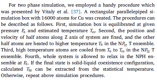
I’ve included my latest coexistence simulation script below, as well as a snippet of the implementation I am attempting to follow (outlined in Zou, et al. 2019). Other than equilibrating the whole system in NVE instead of NPH, have I matched their equilibration procedures? Are there any other oversights in my implementation?
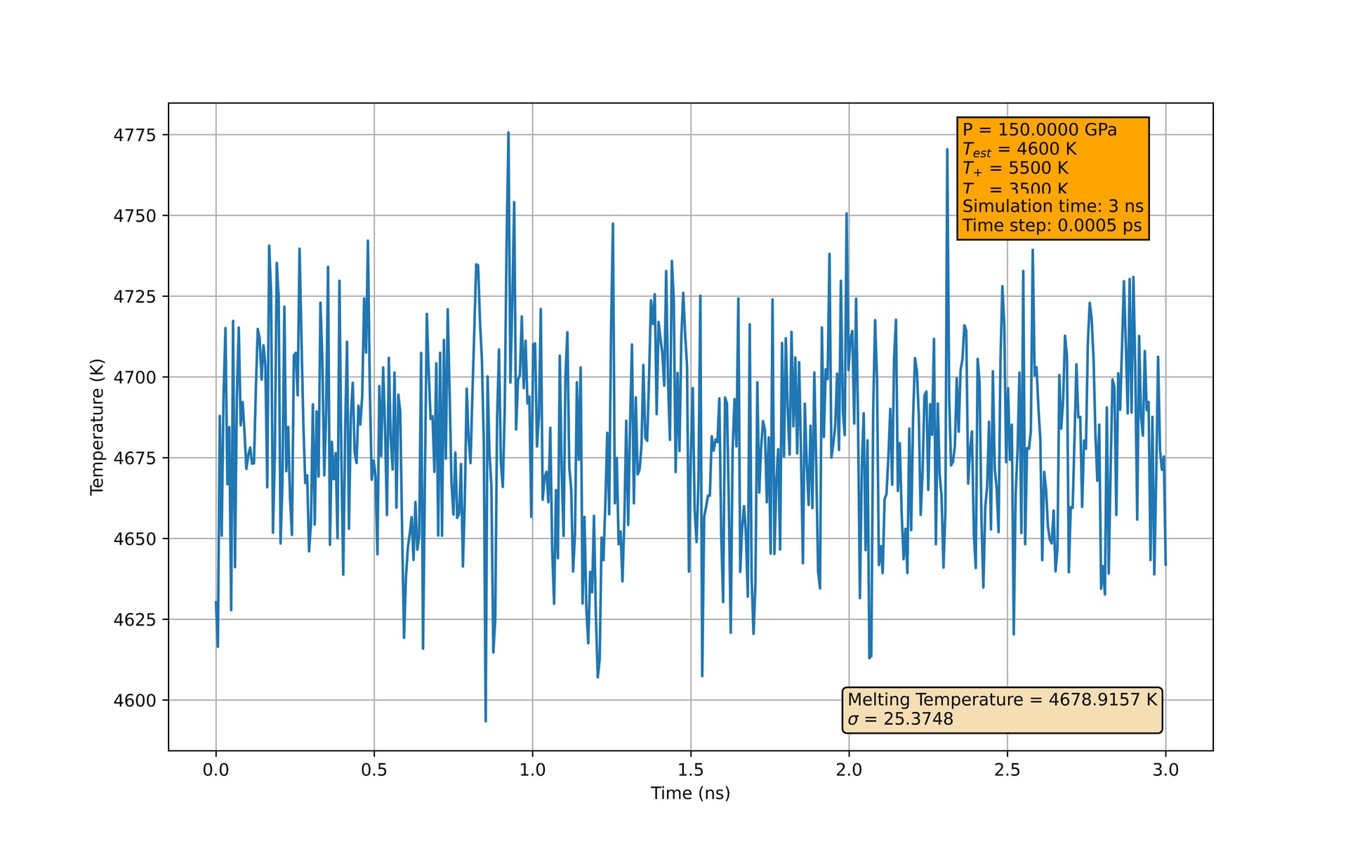
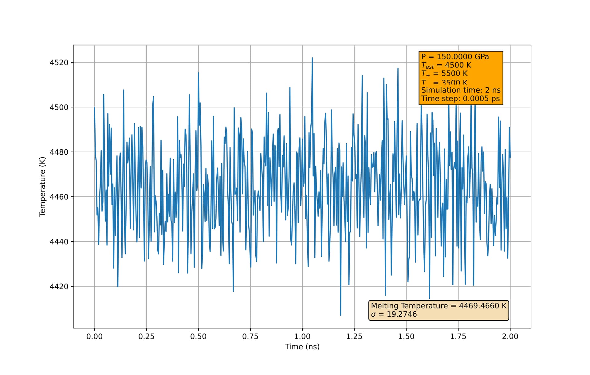
At 1 bar, I am finding a melting temperature of 1350 +/- 8 K, approximately 30 K higher than what was found in Zou, et al. Additionally, at higher pressures, the melting temperature I extract from the final configuration seems to depend strongly on my initial estimate of the melting temperature. In my script below, at 150 GPa, if I change ‘tempMelt’ to be 4500 K instead of 4600 K, I will extract a melting temperature much closer to 4500 K than 4600 K. This holds even using longer equilibration times.
Again, this seems to be only at higher pressure. At 1 bar (other than the thirty-degree difference in estimated melting temperature), the simulation exhibits the expected behaviors, converging to 1350 K regardless of the ‘tempMelt’ assignment (given sufficient equilibration time). I am using the same potential outlined in the paper, and as far as I can tell, have matched their implementation. Just looking to see if anyone more experienced with these simulations can point out any oversights I made. I’ve also included two figures which may help illustrate this concerning behavior.
Some pretty fundamental statistical mechanics shows that (1) different ensembles will give equivalent expectation values only in the thermodynamic / Gaussian-distribution limit; (2) even in that limit their fluctuations will frequently be different. As an example, the average total and kinetic energies are equivalent in (large enough) NVE and NVT ensembles; but the fluctuation of total energy (obviously) and kinetic energy (less obviously) differ in both ensembles regardless of size.
As such I would not assume that an nve run can replicate results from the NPH ensemble unless proven otherwise.
On the other hand, a difference of 20K in a quantity of 1530K is a difference on the order of 2%. Perhaps that is an acceptable accuracy (perhaps not). Do not underestimate the standard error in your estimate: successive snapshots or printouts are usually somewhat correlated; therefore, one cannot naively invoke the CLT and divide standard deviation by the square root of “observations”. The number of uncorrelated observations is roughly the trajectory length divided by the correlation time (for a more rigorous and conservative method one should determine convergence of the block standard error).
That typically indicates non-convergence – your system has not explored phase space enough to truly sample relevant energy minima, instead staying too close to its original configuration. (You have to figure out whether this explanation makes sense for your particular technique.)
As @srtee stated your procedure is different from what the paper’s quote mentions. Coupling to a barostat allows for enthalpy equilibration which is not the same as energy equilibration especially when doing melting simulations (basically any phase change). Since you might be working at different pressure, I have no idea on what you’re comparison with the paper concerning the melting T is worth. Did you look at a P-T diagram for your system? What value do you expect? How does the bulk system behave above and below that temperature and pressure?
Also it is very hard to give a proper comparison of what is correctly done with regards to their work and yours without the full paper to know the calculation details. But that part of the discussion provides better insights with face to face conversation and description of what you wanted to do in your script at each step and direct comments on the paper rather than us going through your inputs trying to guess what you were trying to achieve.
Attempting another implementation of solid-liquid coexistence… Anisotropic barostat means pressure is held constant only in the specified direction(s), right? In the case of a two-phase simulations, is it correct to say that an anisotropic barostat is applied as a way of permitting the system to relax in the direction normal to the solid-liquid interface?
Anisotropic usually means that all directions can relax independently (as in not isotropic). If you let only one direction relax and hold others constant, one usually states explicitly which direction is kept free to relax. Technically speaking, that is anisotropic, too, of course.
In a two-phase/coexistence simulation, what is the purpose of heating half the atoms to a higher temperature and then immediately cooling them back down to the estimated melting temperature? To reduce simulation time? Why not skip the cooling and equilibrate all atoms in NPH/NVE immediately after heating?
If I first equilibrate all atoms at an estimated melting temperature of 1400 K and then heat half of the atoms (denoted ‘liquid’ here) to a higher temperature, say 1800 K, in an NPT ensemble, does it matter which of the following thermostats I use?