Movement of COM in the MD simulation of 3D system consisting mobile and rigid molecules

Dear LAMMPS community,

I simulated a 3D IL system containing HF in its formulation (i.e., fluorohydrogenate ILs). MD simulation of HF has been a topic of debate since 1980s and even before! Among all, the OPLS-based TIPS model suggested by Prof. Jorgensen (https://doi.org/10.1080/00268978400100081) showed to be a reliable one. In this model, a dummy atom, which is only a charge carrier, is added between the H-F bond (0.14 Angstrom from the F atom). The charges and LJ parameters are:

H +0.705 0.0 (A) 0.0 (kcal/mol)
X -1.410 0.0 (A) 0.0 (kcal/mol)
F +0.705 2.984 (A) 0.1505 (kcal/mol)

To model within LAMMPS, the whole molecule (consisting of three atoms, F, H, and X) has to be rigid (i.e., GROMACS seems to have a command in which you can define a virtual site in a molecule without needing to rigidify the whole molecule). When modeling a liquid HF alone rigid, the experimental results are replicated seamlessly. When using this rigid HF model with a pair of IL cations and anions, the density replicates accurately, but visualizing the trajectories shows the movement of the center of mass of the simulation box!

Do you have any interpretations of the reason behind the movement of the center of mass? Does this originate from the combination of rigid-mobile molecules in the system? Is this something I should worry about?
Can I neglect this movement and calculate solvation and transport properties (by subtracting the drift in the COM)?

Thank you in advance for your help.
A

It’s hard to tell if you don’t show the input deck. LAMMPS can execute very different simulations, so everything can happen if you mix enough commands.

There can be multiple reasons for this. It is impossible to speculate without knowledge about your system and setup.

You are not the first person reporting this.

Yes, a center of mass drift adds to the kinetic energy, but a typical bulk MD system should be translation invariant. The thermostat algorithms usually take this into account and thus a drift removes kinetic energy from the relative motions of the system. In the extreme case, this can lead to the system freezing and the drift accelerating massively, leading to the so-called “flying icecube syndrome”.

Only when it is so small that it is negligible. Since you are noticing it, it is probably too large to be ignored and it will likely accelerate.

Hello,
Thank you for the quick reaction to my query. Sorry for the absence of the complementary files. Attached I have enclosed the input and data files. Please let me know if you need output trajectory or log files also. I will upload them on Google Drive and share the link.

To equilibrate the system, I started from a lower density, fix rigid/npt, fix nvt (on the mobile species) to find its equilibrium density at 300K and finally a course of anealing procedure to ensure the mixing quality. The center of mass of the box start moving from the very initial step!

appreciate your help and consideration.
Regards,
A

in.lmp (8.0 KB)
c2c1im-FHF-1.lmp (3.7 MB)

This is not unusual since the rigid body constraints may lead to unexpected net momentum when the velocities are initialized randomly.

You can easily remove that center of mass momentum after the system has somewhat equilibrated by using a velocity all zero linear command. At the point it is probably best to write out a data file and then start with a new input from there or issue a clear command, so that everything is cleanly re-initialized with the center of mass momentum corrected.

Hello Axel,
Thank you a million for these comprehensive explanations. Yes, this COM movement is too large to be ignored.
Do you believe this “flying icecube syndrome” is a result of a deficient thermostat?
Do you think “fix momentum” could be a cure for this? or is this only erasing the question while the problem still exists?

I am a little unsure if I am missing something in my input file.

Many thanks,
A

c2c1im-FHF-1.lmp (3.7 MB)
in.lmp (8.0 KB)

I see!
Thank you very much for the hint!
You mean after applying the “velocity all zero linear” command after equilibration and generating a data file, drift in the COM will not happen anymore!
I will test it and keep you posted very soon.

Many thanks,
A

It is most commonly due to imperfect initial system geometry and equilibration protocol.
Starting from high potential energy configurations means that the initial MD steps have a large error.

There is always a possibility of a small drift forming during MD simulations due to the non-associative nature of floating-point math. Once it is there it is next to impossible to have it dissipate, it will usually increase. Including a barostat will accelerate that, since it creates more numerical noise and thus more errors since positions are converted from real to fractional several times in each MD step.

It is a hack, not a workaround and it has no impact on the rigid body integrators since those maintain velocities for the rigid body translation and rotation so and changes to the velocities will be overwritten after they update the atomic velocities during time integration. That is why it is important to re-initialize them after you make a change to the atomic velocities.

It is better than using fix recenter which will not affect dynamics but just remove the drift after the fact.

No, it can happen again. But it should remove the impact of the most common source of the COM momentum. There are other possible causes like too large a timestep (rigid body integrators can be rather sensitive as far as the rotation goes, especially if the rigid body is not close to spherical in shape). This is where fix shake shines. Unfortunately, it can only be applied effectively to a limited number of cases.

Also, it is useful to dump the unwrapped coordinates to visualise the drift, e.g.

dump TRAJ all custom ${fd} ${out0}.lammpstrj id mol type element q xu yu zu ix iy iz

Thank you very much, Axel, for the comprehensive explanations!
I will re-check several items, do some tests, and keep you all posted of the outcome!

Many thanks,
A

copy that, Otello!
Thank you!
Keep you all posted.
A

Dear Axel,

First of all, I would like to thank you for your tips and instructions. After the above discussions, I searched “flying ice cube syndrome” within the LAMMPS forum and found several threads! The journey was very informative.

I am just posting to report back my experimentations on the case and share the results with the LAMMPS community for future reference. Meanwhile, your final comments on my queries would be very much appreciated and illustrative.

First, I applied the following revisions to my model:

  • Excluding intra pair interactions within rigid-body molecules (Warning: “Neighbor exclusions used with KSpace solver may give inconsistent Coulombic energies,” due to long-range solver via the kspace-solver),
  • Delete bonds, angles, …, within rigid-body molecules,

I further separately computed the temperature of mobile and rigid groups after subtracting out the COM velocity of each group using “compute temp/com,” and then using “fix_modify temp,” the fix temperatures were asked to be modified based on each group’s compute. As also noted in the documentation, “compute temp/com” substracts out constrained DOF due to different fixes (i.e., “fix shake” and “fix rigid” in our case), and consequently, the temperature of groups is computed more correctly.

Q1: The latter modifications led to a 4% increase in the density of the bulk system after NPT when compared to the non-modified fixes! Regardless of whether the revised density better replicates experimental results or not (i.e., experimental outputs are very limited for this system, we expect our own experimental characterizations to pop up soon), is it technically more accurate to modify each fix temperature when we have a mixture of mobile-rigid molecules in a system?

Applying the above modifications (plus reducing the timestep, …), the movement of COM still existed. Therefore, I implemented other remedies suggested by you above and in the other threads. The MD code included 1 ns NVT at lower density and then, 1 ns NPT to find the equilibrium density of the system.

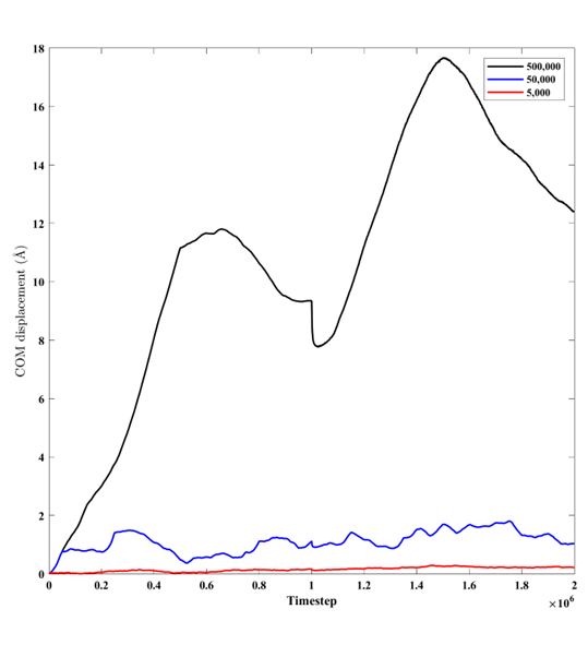
1- velocity zero linear

I called this command with different frequencies within the equilibration phase. The displacement of COM is shown below. As seen, this velocity zero linear command needs to be recalled at finer frequencies for a shorter displacement of overall COM!

I further implemented your recipe for writing a data file after the system reached a somewhat equilibrium (obtained for the above system after applying velocity zero every 5000 steps), and then cleanly re-initialized an MD simulation using the datafile. The movement of COM started again! So, it seems that the COM of the system containing small rigid HF molecules will not stop moving without frequent modification of velocity distribution!
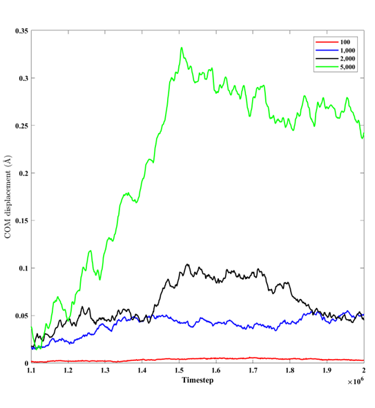
2- fix momentum linear rescale
I read in one of the previous threats that you warned about the frequency of calling fix momentum, in a way that calling fix momentum in every step could make matters worse since this enforces truncation to the floating point resolution, and thus creates noise. In contrast, applying fix momentum every few steps allows some cancelations of the errors due to the coarseness of floating point numbers and non-associative summation. Therefore, I examined the effect of different frequencies on the movement of COM in the system. As seen, even the calling frequency of 1000 for fix momentum can efficiently cancel the net momentum on the COM of the system.

Q2: Upon the explanations/results above, is it technically acceptable to apply “fix momentum linear rescale” during the course of MD equilibration and production runs? Does the command alter the dynamics of the system hugely?

i.e., I am thinking of performing the production runs under NVE; therefore, I think the COM won’t drift drastically in the absence of thermostats. In this case, we might not need to apply fix momentum for the production runs.

Thank you, once again, for all your support.
Regards,
A

fix momentum with linear rescale conserves the total kinetic energy of a system by transferring the kinetic energy of COM movement (relative to box frame) to the interparticle translational degrees of freedom.

This is not generally correct since kinetic energy is generally not conserved. As a simple thought experiment, consider a train as it arrives at a train station, comes to a stop, picks up passengers, and starts moving away:

  • To a physicist at the train station, the kinetic energy of the train decreases to zero and then increases to a constant amount.

  • To a physicist passenger staying on the train, the kinetic energy of the train is zero throughout.

But both of them would agree on the train’s temperature and both would expect largely the same physics (except for when the train is accelerating or decelerating).

Of course, with specific justifications, it could be correct to move the COM KE back into the thermal degrees of freedom. That’s a very system-specific question though.

The purpose of this step is to counter the unphysical cooling effect of a thermostat on a drifting system.

As the drift builds, the temperature compute will include this in the computation of the temperature which means that the kinetic energy in the frame of the system will be reduced. In the extreme case it will lead to a frozen system speeding through space. Of course, the purpose of fix momentum is to avoid even getting near that state, but you will still have a bias toward cooling the system, if you won’t put back the kinetic energy, that the thermostat has removed.

2 Likes

Thank you for clarifying that, Axel! Those were very illustrative. And I think calling fix momentum not on every iteration avoids further unphysical incidents.

Just to wrap up this thread, would you please share your comments on the application of fix_modify temp separately for mobile and rigid bodies?

Q1: The latter modifications led to a 4% increase in the density of the bulk system after NPT when compared to the non-modified fixes! Regardless of whether the revised density better replicates experimental results or not (i.e., experimental outputs are very limited for this system, we expect our own experimental characterizations to pop up soon), is it technically more accurate to modify each fix temperature when we have a mixture of mobile-rigid molecules in a system?

Many thanks,
A

Thank you very much, Shern, for sharing your ideas. Axel’s complementary explanations were clarifying.
A

It is not at all clear what you mean by this.

It is a kind of silly question. However, I meant when we have a combination of rigid and non-rigid bodies in our system, especially with some movement of COM, is it better to define each fix temperature based on its group temperature (after subtracting out the center-of-mass velocity of the group) or let the fix nvt (npt) use its own compute style “temperature”?

Scenario 1:
fix 1 mobile_group nvt temp 300 300 100.0
fix 2 rigid_group rigid/nvt molecule temp 300 300 100.0

Scenario 2:
compute temp_m mobile_group temp/com
compute temp_r rigid_group temp/com|

fix 1 mobile_group nvt temp 300 300 100.0
fix 2 rigid_group rigid/nvt molecule temp 300 300 100.0

fix_modify 1 temp temp_m
fix_modify 2 temp temp_r

Scenario 2 is probably a more correct approach. Right?

Regards,
A

Not necessarily. The center of mass for each group may fluctuate and this will make the thermostat ignore that. Also, if you use this setting you must not use the rescale option of fix momentum, since you already compensated for the center of mass contribution to the kinetic energy and using rescale would add this kinetic energy twice.

Crystal Clear!

Thank you very much for all the instructions and hints, Axel!

Regards,
A