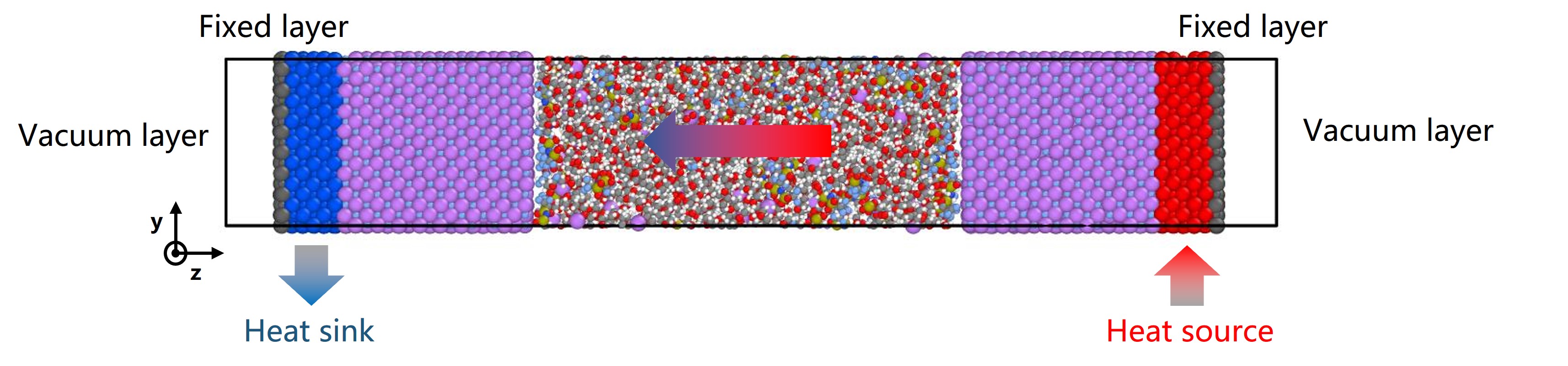
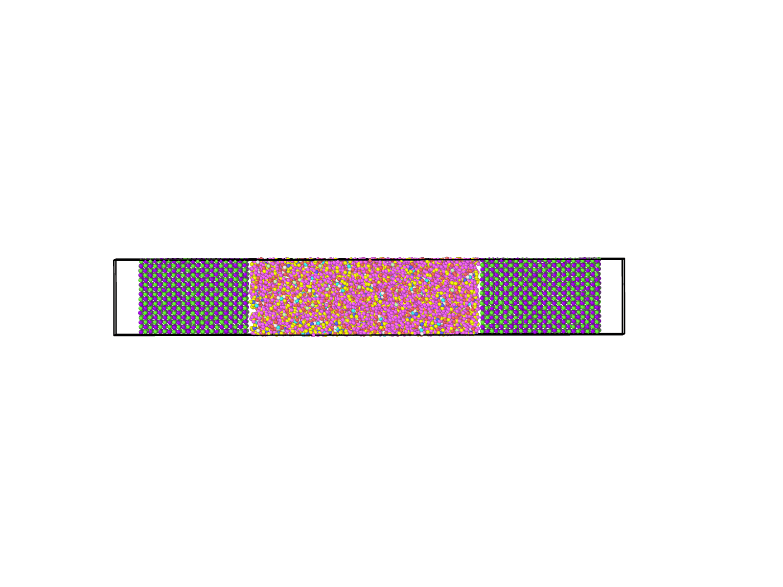
I’m running into a problem where energy is not conserved when I try to calculate the interfacial thermal conductivity using NEMD with Langevin thermostat. My model is shown as the image below, which consists two LiF blocks at each ends and PEO(LiTFSI) electrolyte in the middle.
The atom interaction in LiF part is described by Buckingham potential, while the PEO(LiTFSI) part is described by OPLSAA force field. The non-bonded interaction between LiF and electrolyte is described by Universal force field. It’s worth mentioning that I am not that confident whether this setting of atom interacton is correctly presented in my in.script which is attached at the end of this post. If you have any relevant experiences, please check my in.script for me. Thank you very much!
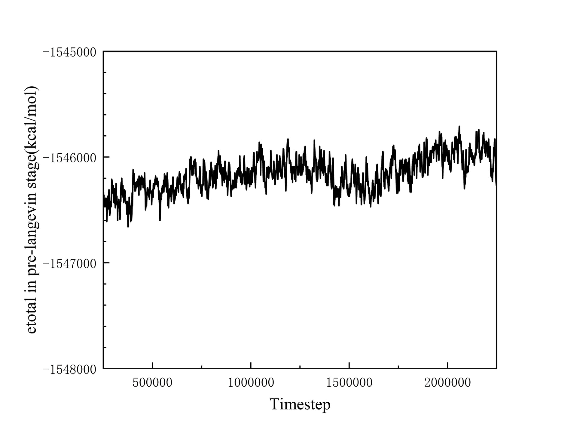
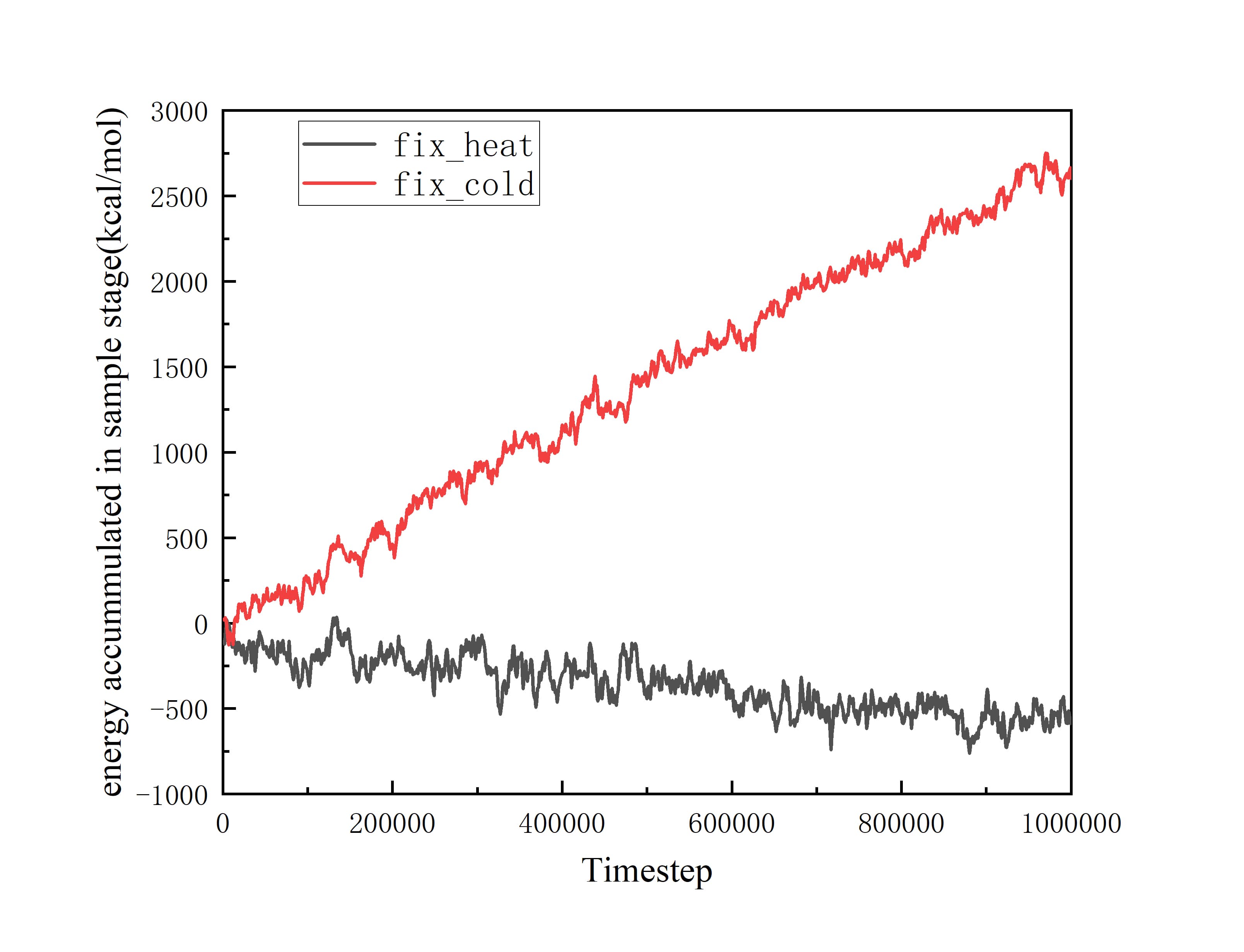
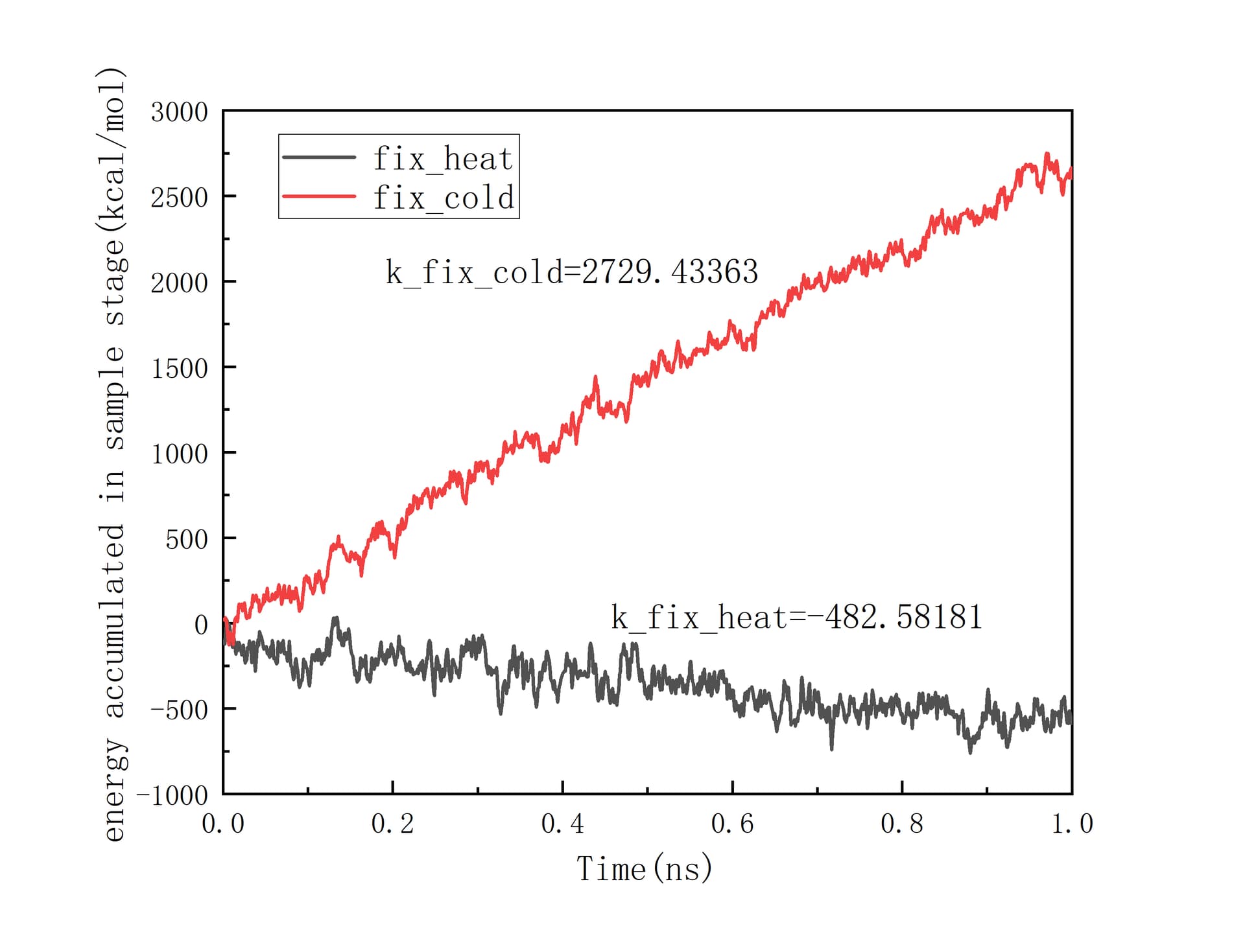
After fully relaxed by a series of NPT and NVT ensemble, I set Heat sink, Heat source, Fixed layers and vaccum layers in the position showed in the picture above. Simultanenously, the part that goes from heat sink to heat source is set as main group to product various thermaldynamic data. Then I did a pre Langevin thermostat for 2 ns(timestep is 1 fs) , making the gourp reach equilibrium. I collect the total energy of system and the accummulated heat injected or extracted by Langevin thermostat. They are illustrated as below:
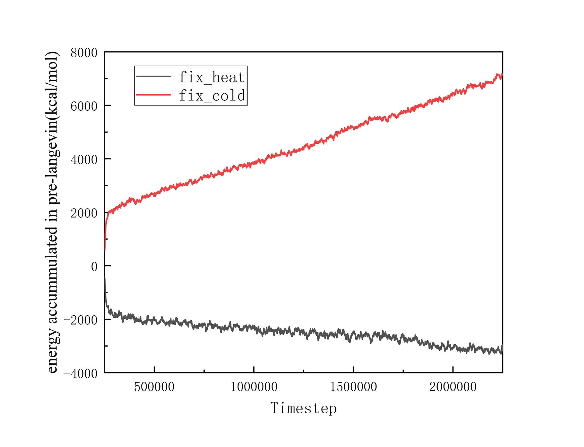
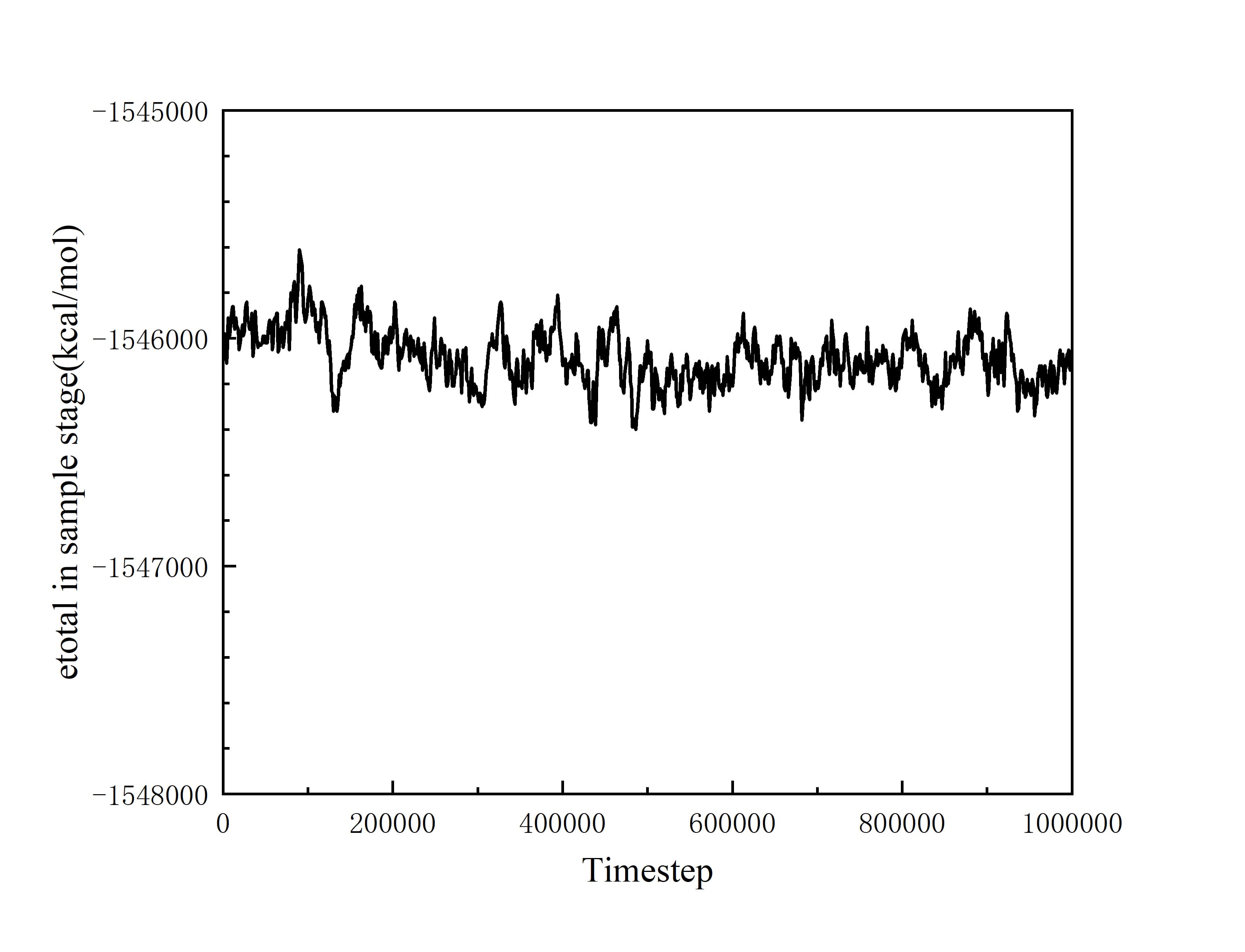
At this time, the phenomenon of non-conservation of energy has begun to appear. And I continued to excute Langevin thermostat for 1 ns to product more reliable data. Revelant pictures are also attached below:
The difference between solpes of fix_heat and fix_cold is too large to ignore. I can’t precisely calculate the heat flux through the interface based on these data.
So my question is how to explain this non-conservation phenomenon and how to fix it?
Dump file of Langevin thermostat stage, temperature distribution and in.script are provided as supplementary information.
Any suggestion is highly appreciated from the bottom of my heart.
Your script is very complicated as a lot of things are going on and it is hard to pinpoint any LAMMPS problem, if any, with so many commands.
However some things already bug me in what you show.
Is there any reason to use lj/cut for cross interactions when you use long coulombic interactions for all your types? This looks completely bogus to me.
The difference between solpes of fix_heat and fix_cold is too large to ignore.
Why ? They represent the cumulated energy from both fixes. Is there a reason for them to be linked at the moment? What are the values? Did you compare them? Should readers guess them based on your graph?
Then I did a pre Langevin thermostat for 2 ns(timestep is 1 fs) , making the gourp reach equilibrium.
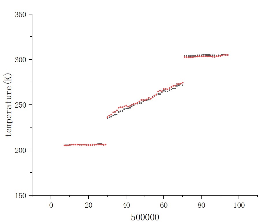
How do you know? Your temperature graph indicates gaps in temperature between your interfaces. This makes me believe your system has not reached stationary state.[1]
Dump file of Langevin thermostat stage, temperature distribution and in.script are provided as supplementary information.
From my reading of your post, these are actually what gave me insights of your issue. This should be central to the info you provide to readers, not peripheral or provided as “Supp. info.”.
Here are some general thoughts to help you presenting data:
Your figure values do not correspond to the one provided in the input script. This deserves attention or a comment. Did you use a different simulation to produce it? It seems very weird to have all your temperature below 300K when it is apparently the average between your heat and sink.
This is not a dump file. This is a gif, and it is as useful as a kitten picture since it does not depict precise event you would like to draw our attention to. It is wasting readers’ attention.
Your graph has no legend, no title, nor label on the X axis (what does (500000 represent?). My reading is based on guesses from the input file. It is not self sufficient which should be the point of plotttes data.
Which is NOT equilibrium since your are doing N(on)E(quilibrium)MD… ↩︎
Firstly, thanks so much for your kindness sparing your precious time to answer my question.
And I really apologize that I did not emphasize the main content, making my post unexplicit for readers.
The idea of using lj/cut comes from a paper about “Li-PEO interfacial thermal conductance”. It said using universal force field to describe the non-bonded interactions across the interface. And my understanding for universal force field is lj/cut pair style, where the specific parameters are exactly from paper about this force field. As for the ‘long’ coulombic interactions, this pair style is from OPLSAA force field, where the parameters generated by the software moltemplate .
I am sorry that I have not annotated the specific values of the two slopes in the graph. The slopes of fix_heat and fix_cold are -482.58181 and 2729.43363 respectively with units of kcal/mol/ns. Normally, they should have opposite signs, but close absolute values. So their big difference in absolute values indicates the “Non-conservation of energy”, which is exactly my confusion.
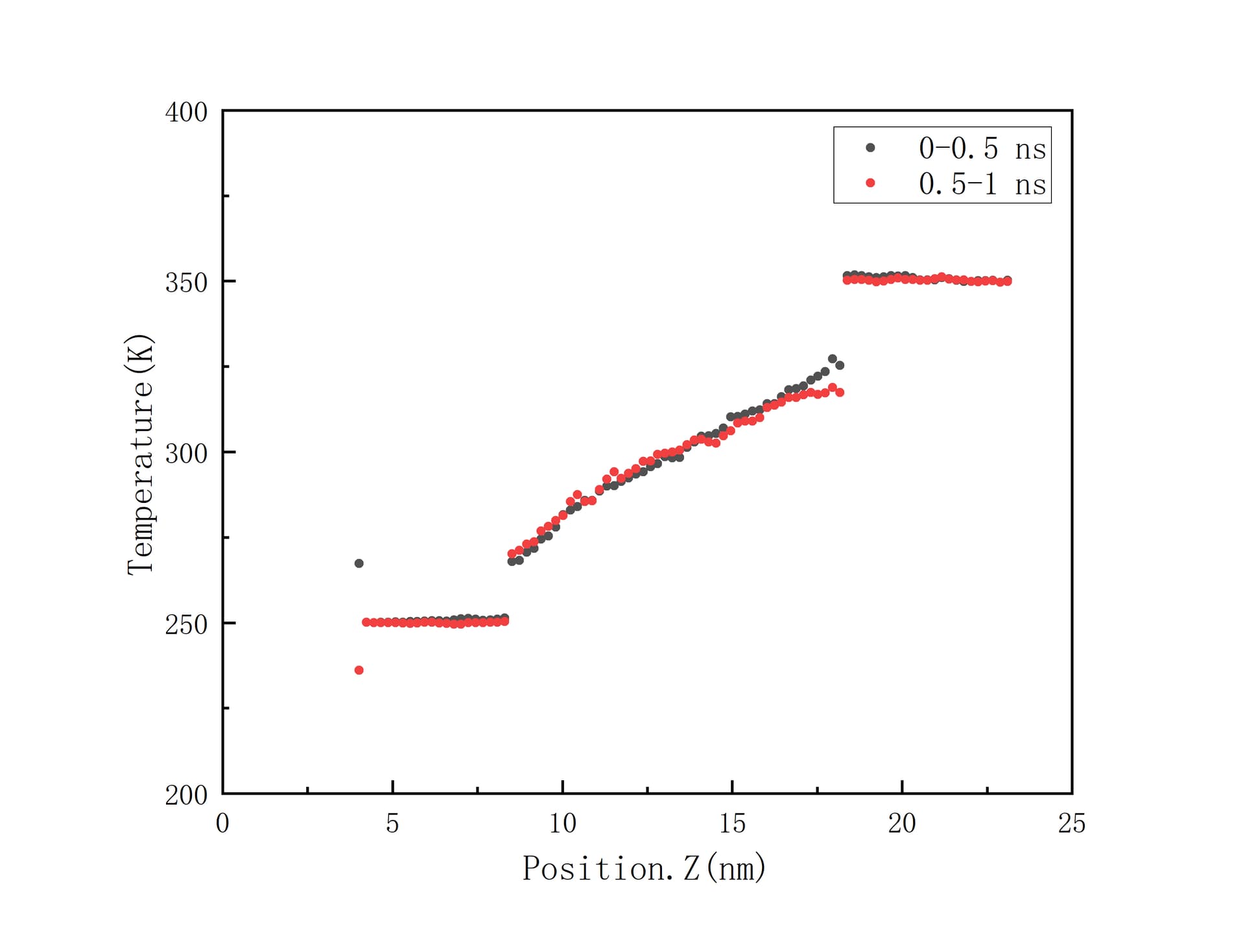
In my opinion, the gaps in temperature between interafaces means the interfacial thermal resistance exists. And my original thought of “pre langevin thermostat” I said is to prepare for the final langevin thermostat phase where convergence data is collected. Now I attach the new temperature distribution graph below. The black dots and red dots represent averaged data during 0 to 0.5 ns and 0.5 to 1.0 ns, repectively. The two prominent black and red dots at the far left of the figure should be the result of too few atoms being counted in the chunk region.
I’m sorry I didn’t emphasize the information, especially for the in.script.
Thanks for your kind suggestions. The temperature distribution figure is updated above, and sorry to make you and other concerned readers confused about the conflicting infomation I offered.
I originally thought the dump file is not that important for tacking my problems. But I will attach it at the end of this reply.
Thanks again for your attention and patient reply. I really appreciate it if you could offer more valuable experiences tacking this kind of Non-conservation problems.
UFF includes charges. See the original paper section 2.F. As is, they are not taken into account at all in your simulation for cross interactions.
What makes you say that? Honest question. On one side you have a sink that receive a certain amount of heat from your central part, on the other you have a source that gives heat to this very central part. The transfer will depend on thermal conductivity but also temperature. They will also depend on your langevin parameters. Why should they be the same with different temperatures out of steady state?
You are doing NEMD simulation. What do you think should happen between the transition from equilibrium to steady state?
Does it? What supports this opinion? Science is not about making guesses but also justifying them. I see no reason why a gap in temperature should exist between two molecular system in direct contact in a steady state. This makes no sense from a thermodynamics point of view. Where would the energy kinetic go? This should be discussed with your advisor because this is about the physics of the model.
By the way:
This commands only makes 2 averages during your acquisition phase which is very low to make statistics out of data. You loose a lot of information that you could reconstruct easily, with more regular writing, and you could compute variances and see the time evolution of your profiles. In the same way, a dump file with only 10 snapshots containing only particles coordinate is very low in information. What do you want us to make out of this?
Last point:
The graph was not only updated, these are different data. Where they from a different simulation than the first one? Where are the first one from then? These are questions more for you than really important to answer here, but wonder what you wanted to ask by providing this in the first place. My other points are more important.
I really think this is an issue you should discuss directly with your advisors and look into the relevant literature for NEMD simulation setup and analysis.
@Germain – the temperature jumps are known and normal for heat flow across the nano-interface. The interfacial thermal resistance (ITR), or “Kapitza resistance”, comes from phonon mismatch between materials, and arises as the solution for the Fourier heat equation across a discontinuity in the thermal conductivity.
It is certainly obscure – I did work with another postdoc last year on quantifying ITR for MD simulations of carbon nanotubes and whether constant potential molecular dynamics affects that. Otherwise I wouldn’t have heard of ITR before this either!
You’re right that a temperature jump across directly-contacting surfaces violates equilibrium thermodynamics – but the heat flux across the surface means the system is NOT at equilibrium. (With zero net heat flux, there would be zero temperature gap, and thus identical temperature, as required.)
@yikang – you are simply trying to debug too many steps at once in your script. Please break your simulation procedure up into discrete steps and make sure you have sensible results at the end of each step. If you do not know what is sensible for the end of each step, then that is a big problem in itself.
Besides that, I still think a jump from 250K to 350K is way too large. Most materials do not have a constant thermal conductivity across such a large temperature difference, and as you can see for yourself, as the polymer equilibrates (remember, polymers have longer equilibration times because their molecules are longer and more entangled!), the temperature profile with position is becoming non-linear.
You should introduce your “vacuum gap” RIGHT AT THE START of your simulation procedure, unless there is some compelling reason for you to waste several nanoseconds of simulation time effectively equilibrating a completely different system. (A system that is discontinuous in the z-axis has completely different phonons from an infinite periodic discontinuous system.)
Along the same vein, you should use boundary conditions that are non-periodic in z (boundary p p f), and use slab-corrected long-range electrostatics (kspace_modify slab 3.0), because:
A large enough temperature gradient across a fluid induces an open-circuit emf due to the change in thermal ionic and dipolar ordering (a “Seebeck effect” – https://pubs.acs.org/doi/10.1021/acs.jctc.3c00760).
It stands to reason that in a sufficiently ionically-conductive polymer, the Seebeck emf will lead to a cell-long electric dipole, and without slab corrections, the dipole will mutually-reinforce across repeating cells leading to spurious long-range ordering.
I would rather mirror the system instead of using the slab correction, so that you have two middle regions with a vacuum/2-"cold"-"gradient"-"hot"-vacuum-"hot"-"gradient"-"cold"-vacuum/2 kind of setup. The slab correction will make kspace much more expensive (you need to process 3 times the volume and the cost scales N*log(N) with the volume), while with mirroring you have only double the volume and have double the statistical sampling (but also double the computational cost for Pair and Bond etc.).
Indeed – if @yikang doesn’t need the vacuum (and I can’t see why they do, but that’s specific to their final use case) they should be able to omit the vacuum gaps altogether and simply embed one heating region and one cooling region in the middle of each of their LiF blocks.
That would mimic the Muller-Plathe method, and if it hasn’t been tried before in Kapitza resistance simulations it would be an actual (albeit minor) methods innovation.
Thanks a lot for your enlightening suggestions, which give me a new perspective to think about this problem.
The 100K gap is set based on the fact that there are 2 interfaces existing in this model, sothat the temperature jump beween “cold” and “heat” region needs to be big enough to creat two distinct temperature gap for calculating “ITR”. The vacuum layer was originally used to isolate the two sides of the model from atomic interactions due to periodic conditions. But I will reset the temperature jump and revisit the role of vacuum layers and the timing of adding them, considering your suggestions.
A quick Google search (“kapitza resistance molecular dynamics”) shows a paper (https://www.sciencedirect.com/science/article/pii/S2468023022004540) detailing how ITR changes with ΔT, implying that (in practice) too-large ΔT may give you results that are not applicable at your actual operating temperatures.
In my previous literature research, I did see many articles on interface thermal resistance that set the temperature difference to 100K or even larger. And I thought that is a proper setting. I haven’t looked into the literature that shows that the thermal resistance of the interface changes with the temperature difference or anything like that.
That’s a novel idea to me. Thanks for your supplement !
Please double-check the literature – and be careful that you aren’t taking too much inspiration from solid-solid interfacial studies when you’re effectively studying a solid-fluid interface in your studies.
Hey yikang;
i wonder how did you kept the layers of materials seperate during NPT NVT how did you pack them and how did you keep the interface clear so they do not mix with each other…
I would recommend that you start a new thread with your questions, as reopening old threads will make the flow of posts difficult to understand for future readers.
Additionally, do make your questions more clear and concrete. “How did you do XYZ?” is often very difficult for us to answer clearly because we do not know what you have or haven’t tried and therefore what advice we should give.
The easiest questions for us to answer are: “I thought that doing ABC would give results X, based on my understanding of P physical / mathematical principle / statement from the documentation, but I got results Y instead, and I would like to know why.”
Not only does this give us very clear starting points to make suggestions for you to try – these questions are also highly analogous to the kinds of questions reviewers will eventually ask you, so the answers you get now will be fruitful later on.