Open Review

Hello everyone :slight_smile:

I am using this post to carry out a participated peer review of a paper, which I hope to publish in the next few months. It is about a coarse-grained force field for LAMMPS based on ellipsoids decorated with point charges and connected by directional bonds. Its main features are:

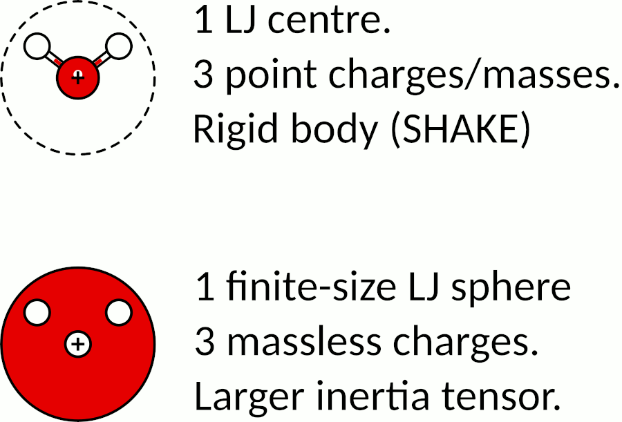
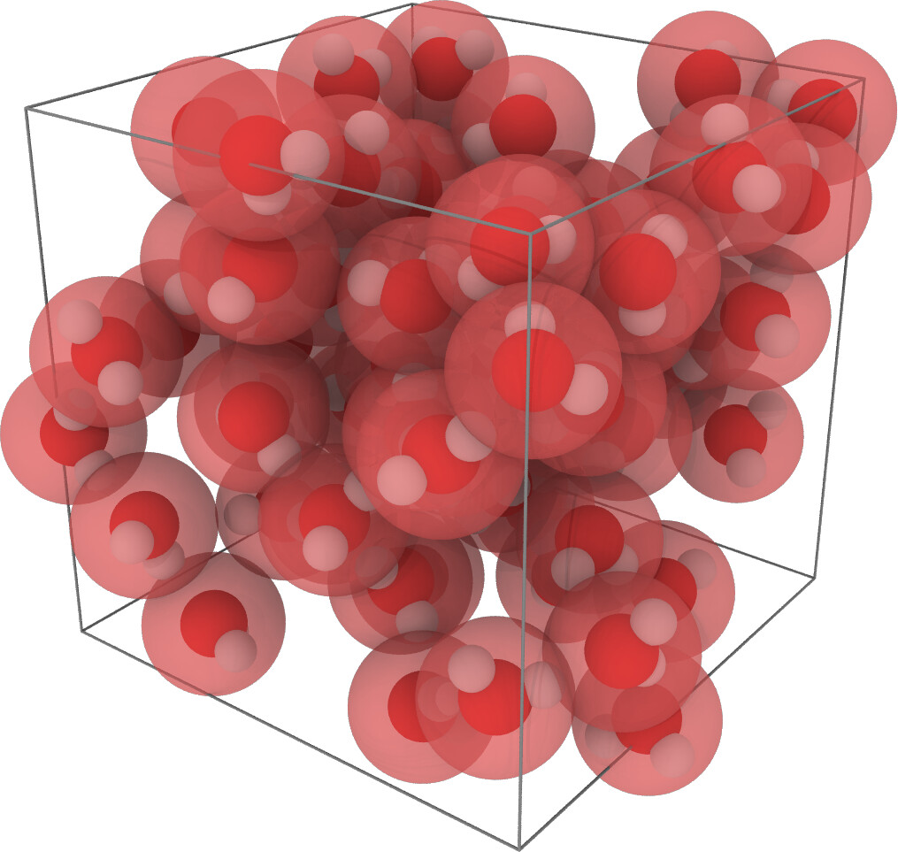
  • It reproduces the excluded volume of molecules ( → overlapping ellipsoids).
  • It includes long-range electrostatics, yielding good condensed-phase properties.
  • It can be back-mapped to atomistic coordinates without losing structural information (as the CG beads are finite-size particles, they also have a quaternion describing their orientation).

The first implementation was based on lammps-30Oct19 as a hybrid pair_style. Here is the accompanying paper: MOLC. A reversible coarse-grained approach using anisotropic beads for the modelling of organic functional materials (2019).

I left academia after publishing this paper, and these days I am a scientific consultant. However, I keep working on the MOLC model as I am pretty confident about the quality of the resulting simulations. I am preparing a paper describing a new parameterisation strategy, plus bits which are of general interest to the MD community (e.g. a new compute for the intermolecular energy of force-fields with long-range electrostatics).

Meanwhile, the MOLC model has been ported to lammps-2Jun22 and transformed into a pair_style, which is a combination of a Gay-Berne potential plus classic electrostatics with point charges. The original plan was to submit the new code to the main LAMMPS repo after peer review, but the developers would need to audit the code anyway. So I asked directly one of them, as it’s unlike that a referee will have the time and resources to scrutinise the code and verify the consistency of the physical equations.

Let’s take the chance to run a little experiment together. I will discuss the paper’s open issues and technical details in this post. I have asked @akohlmey to referee the paper before submission, and I will include him as a co-author to acknowledge his precious contribution. I have received countless suggestions in this forum, and it is clear that erroneous results can and indeed do pass peer review, especially for very technical subjects. I recently read an interesting post questioning the efficacy of peer review, so let’s try an open review instead. Feel free to share your thoughts on this approach or the scientific aspects.

The paper deals with the parametrisation of linear alkanes. Here is a teaser showing the CG model of n-hexadecane (C16H34) superimposed to the back mapped atomic coordinates: hexadecane_cg_aa

I will post anything specific to the MOLC model here and discuss more general issues on the #lammps forum. Keep you posted!

2 Likes

Looking forward to that.

I know people that this work would interest a lot.

Following the discussion from this post, I take the chance to explain the MOLC model for the “simple” case of water. In this example, a single molecule of water is represented by a finite-size sphere decorated with point charges. In the MOLC model, the electrostatic interactions are accounted for via virtual sites acting as point charges. The charges are defined in the molecular frame of reference, while the parent spheroid also includes a short-range Gay-Berne potential. With this setup, the CG model of water is computationally almost identical to the reference atomistic model, as shown in this cartoon:

The water model is a fantastic example to test the effect of how the pressure is computed, as we can use the corresponding atomistic model as a reference, see the attached input deck:
water_aa.tgz (75.0 KB).

The following script creates and equilibrates a sample of CG water. The pressure is computed with the translational temperature replacing the default one in npt/asphere.

# TIP3P water: use the pressure translational.
variable run    string water01
variable dt     equal 5
units		real
atom_style	ellipsoid
dimension	3

# Set-up the sample.
lattice         sc 3.2
region          box block 0 10 0 10 0 10        
create_box      1 box
create_atoms    1 region box
set             type 1 mass 18.0152
set             type 1 shape 3.188 3.188 3.188
set             group all quat/random 154484

# Set-up the force field for TIP3P water.
#  gamma, upsilon, mu, cutoff_global, cutoff_electrostatics
pair_style      molc/long 1 1 1 12. 12.
# Pair coefficients:
# epsilon0, sigma0, eps_x, eps_y, eps_z, n_charges, (xi, yi, zi, qi)_ntimes
pair_coeff 1 1 0.102 3.188 1 1 1 3 &
  0.000000     0.000000     0.000000 -0.830 &
 -0.756950     0.585882     0.000000  0.415 &
  0.756950     0.585882     0.000000  0.415
kspace_style pppm/molc 1e-4
neighbor	4. bin
neigh_modify	check yes

# Physical observables.
compute q               all property/atom quatw quati quatj quatk
compute diameter        all property/atom shapex shapey shapez
compute temp_trasl      all temp
compute temp_rototrasl  all temp/asphere dof all
compute press_trasl     all pressure temp_trasl
compute press_rototrasl all pressure temp_rototrasl 
variable tcouple equal ${dt}*100
variable pcouple equal ${dt}*1000

# Average T and P.
fix AVE all ave/time 10 50 500 c_temp_trasl c_temp_rototrasl c_press_trasl c_press_rototrasl mode scalar ave running

# Output.
thermo       500
thermo_style custom step etotal evdwl ecoul elong ke pe temp press vol density cpu
thermo_modify temp temp_rototrasl press press_trasl

# Trajectory (ovito will recognise every column by default).
dump TRJ all custom 10000 ${run}.dump &
id type xu yu zu c_q[1] c_q[2] c_q[3] c_q[4] c_diameter[1] c_diameter[2] c_diameter[3] &
vx vy vz angmomx angmomy angmomz
dump_modify TRJ colname c_q[1] quatw colname c_q[2] quati colname c_q[3] quatj colname c_q[4] quatk

# Equilibration and production.
timestep        ${dt}
fix		NPT all npt/asphere temp 300. 300. ${tcouple} iso 1. 1. ${pcouple}
fix_modify      NPT press press_trasl
run		300000 post no
print "Temp_trasl $(f_AVE[1])"
print "Temp_rototrasl $(f_AVE[2])"
print "Pressure_trasl $(f_AVE[3])"
print "Pressure_rototrasl $(f_AVE[4])"
unfix NPT

# Microcanonical.
fix AVE all ave/time 10 50 500 c_temp_trasl c_temp_rototrasl c_press_trasl c_press_rototrasl mode scalar ave running
fix NVE all nve/asphere
run		300000
print "Temp_trasl $(f_AVE[1])"
print "Temp_rototrasl $(f_AVE[2])"
print "Pressure_trasl $(f_AVE[3])"
print "Pressure_rototrasl $(f_AVE[4])"

Run this example using this fork: lammps-2Jun22. With these settings, the simulation is stable and the density is identical to the reference atomistic model, as shown in the comparison:
image

Conversely, if the default setting is used for computing the pressure in npt/asphere, the sample fails to reach the desired density (i.e. it explodes). Please refer to the paper for a more detailed comparison of other physical properties.

A few more comments on the previous post:

  • The MOLC model of water has 6 degrees of freedom even though it is a sphere: the off-centre charges (corresponding to hydrogen atoms) provide the torque.
  • The energy expression for pair_style molc/cut and pair_style molc/long is: \begin{equation}U = U_\text{short}+U_\text{Coulomb}\end{equation},
    where U_\text{short} is the Gay-Berne potential and U_\text{Coulomb} is the standard Coulombic potential.
  • The pair_coeff coefficients are defined for each pair of atoms types I=J. A single set of \varepsilon_i coefficients is specified, which is a bit less cumbersome than the standard Gay-Berne notation. Mixing for I!=J is performed by LAMMPS using the arithmetic rules.
  • The charges are defined in the spheroid frame of reference and specified
    as a list of Cartesian coordinates and charge values. This means that the
    charges are defined as point particles around a spheroid with the centre in (0,0,0) and orientation \mathbf{q}=(1,0,0,0). The charges will follow the position and orientation of the parent spheroid during the simulation. Still, there is no constraint on whether they are positioned well within the repulsive core of the Gay-Berne potential or outside. To avoid lost atoms errors, it is always better to protect the charges inside a repulsive potential, but there may be cases where it may be convenient to exploit this flexibility (e.g. in a rigid body).
  • Water models such as TIP4P or with more charges are natively supported by the pair_style molc, as any number of charges can be specified inside the oxygen sphere.
  • Note that a finite-size sphere has a large inertia tensor than the corresponding atomistic model. So even if the functional form of the pair potential is the same for atomistic and coarse-grained water (in the previous example), some physical observables will be slightly different, typically higher viscosity and lower diffusion coefficients. Which is a bit counter-intuitive for a coarse-grained model :wink:

Also, I am attaching a toy system of 64 water molecules in exactly the same configuration, both in CG and AA coordinates:


This is for debugging purposes. The run 0 command returns the same energy for both models, proof that we are computing the same forces and slightly different torques. Yet, the pressure is very different for both systems:

CG:
   Step         TotEng         E_vdwl         E_coul         E_long         E_bond         KinEng         PotEng          Temp          Press           Pxx            Pyy            Pzz           Volume        Density          CPU
         0  -730.63121      131.1518       4634.9135     -5496.6965      0              0             -730.63121      0             -947.6651      -1664.3816     -1852.6195      674.00572      1911.2405      1.0017348      0                                                         
AA:
   Step         TotEng         E_vdwl         E_coul         E_long         E_bond         KinEng         PotEng          Temp          Press           Pxx            Pyy            Pzz           Volume        Density          CPU
         0  -730.57301      131.19354      4634.9239     -5496.6989      0.0071847542   0             -730.57301      0              28062.747      26875.301      28094.464      29218.476      1911.2405      1.0017348      0            

Here the input deck for both systems:
water.tgz (14.8 KB)

Feel free to ask any question, as this discussion will form the basis for documenting this new pair style. Thank you in advance!

@hothello thank you for finally making me understand the importance of aspherical particles to represent rings in coarse grained models. figure 1 of your MOLC paper was quite informative and illustrative.

now i can see why martini cg force field has such a difficult time representing DNA, which might the reason they’re withholding publication/software for DNA in martini 3, ie. representing the ring structures of AGCT bases with 2-3 cg spheres doesn’t work, a single flattened aspherical bead to represent rings is necessary as it’s done in CG-DNA.

these aspherical particles should to be added to CG-SPICA to properly represent amino acids side chains with rings, ie. Histidine, Proline, Phenylalanine, Tyrosine, Tryptophan.

(https://www.spica-ff.org/mapping/map_protein.png)

I’m glad you found the MOLC paper informative. If you want to see it in action, check out this cheeky video which I have prepared to promote my company. Forgive my accent and focus on the transitions between AA and CG models: they come from simulations executed with LAMMPS.