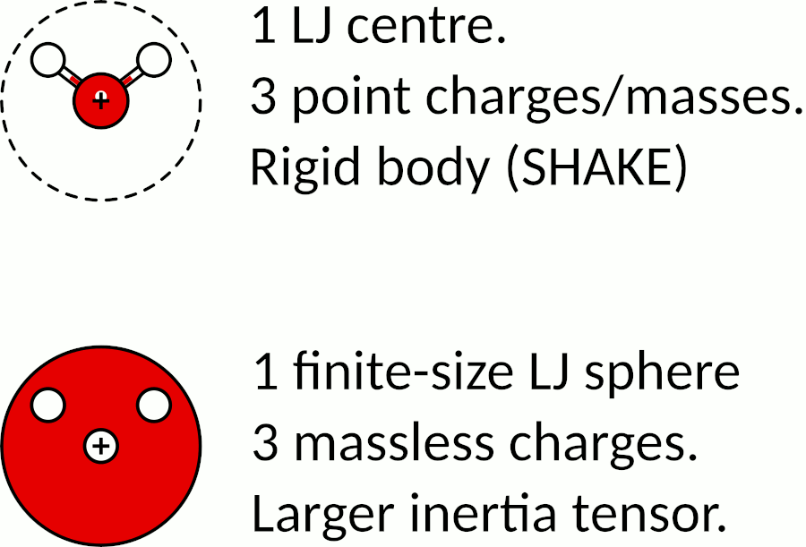
Following the discussion from this post, I take the chance to explain the MOLC model for the “simple” case of water. In this example, a single molecule of water is represented by a finite-size sphere decorated with point charges. In the MOLC model, the electrostatic interactions are accounted for via virtual sites acting as point charges. The charges are defined in the molecular frame of reference, while the parent spheroid also includes a short-range Gay-Berne potential. With this setup, the CG model of water is computationally almost identical to the reference atomistic model, as shown in this cartoon:
The water model is a fantastic example to test the effect of how the pressure is computed, as we can use the corresponding atomistic model as a reference, see the attached input deck:
water_aa.tgz (75.0 KB).
The following script creates and equilibrates a sample of CG water. The pressure is computed with the translational temperature replacing the default one in npt/asphere.
# TIP3P water: use the pressure translational.
variable run    string water01
variable dt     equal 5
units		real
atom_style	ellipsoid
dimension	3

# Set-up the sample.
lattice         sc 3.2
region          box block 0 10 0 10 0 10
create_box      1 box
create_atoms    1 region box
set             type 1 mass 18.0152
set             type 1 shape 3.188 3.188 3.188
set             group all quat/random 154484

# Set-up the force field for TIP3P water.
#  gamma, upsilon, mu, cutoff_global, cutoff_electrostatics
pair_style      molc/long 1 1 1 12. 12.
# Pair coefficients:
# epsilon0, sigma0, eps_x, eps_y, eps_z, n_charges, (xi, yi, zi, qi)_ntimes
pair_coeff 1 1 0.102 3.188 1 1 1 3 &
  0.000000     0.000000     0.000000 -0.830 &
 -0.756950     0.585882     0.000000  0.415 &
  0.756950     0.585882     0.000000  0.415
kspace_style pppm/molc 1e-4
neighbor	4. bin
neigh_modify	check yes

# Physical observables.
compute q               all property/atom quatw quati quatj quatk
compute diameter        all property/atom shapex shapey shapez
compute temp_trasl      all temp
compute temp_rototrasl  all temp/asphere dof all
compute press_trasl     all pressure temp_trasl
compute press_rototrasl all pressure temp_rototrasl
variable tcouple equal ${dt}*100
variable pcouple equal ${dt}*1000

# Average T and P.
fix AVE all ave/time 10 50 500 c_temp_trasl c_temp_rototrasl c_press_trasl c_press_rototrasl mode scalar ave running

# Output.
thermo       500
thermo_style custom step etotal evdwl ecoul elong ke pe temp press vol density cpu
thermo_modify temp temp_rototrasl press press_trasl

# Trajectory (ovito will recognise every column by default).
dump TRJ all custom 10000 ${run}.dump &
id type xu yu zu c_q[1] c_q[2] c_q[3] c_q[4] c_diameter[1] c_diameter[2] c_diameter[3] &
vx vy vz angmomx angmomy angmomz
dump_modify TRJ colname c_q[1] quatw colname c_q[2] quati colname c_q[3] quatj colname c_q[4] quatk

# Equilibration and production.
timestep        ${dt}
fix		NPT all npt/asphere temp 300. 300. ${tcouple} iso 1. 1. ${pcouple}
fix_modify      NPT press press_trasl
run		300000 post no
print "Temp_trasl $(f_AVE[1])"
print "Temp_rototrasl $(f_AVE[2])"
print "Pressure_trasl $(f_AVE[3])"
print "Pressure_rototrasl $(f_AVE[4])"
unfix NPT

# Microcanonical.
fix AVE all ave/time 10 50 500 c_temp_trasl c_temp_rototrasl c_press_trasl c_press_rototrasl mode scalar ave running
fix NVE all nve/asphere
run		300000
print "Temp_trasl $(f_AVE[1])"
print "Temp_rototrasl $(f_AVE[2])"
print "Pressure_trasl $(f_AVE[3])"
print "Pressure_rototrasl $(f_AVE[4])"
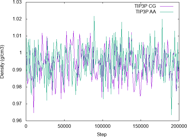
Run this example using this fork: lammps-2Jun22. With these settings, the simulation is stable and the density is identical to the reference atomistic model, as shown in the comparison:
Conversely, if the default setting is used for computing the pressure in npt/asphere, the sample fails to reach the desired density (i.e. it explodes). Please refer to the paper for a more detailed comparison of other physical properties.