Problems with pair table reproducing a LJ potential

Dear all,
I need to use a pair_style hybrid/overlay including a pair_style table to implement a 12-6-4 Lennard Jones potential.
During the energy minimization I receive a lot of WARNING messages which state “WARNING: 1490 of 1801 force values in table are inconsistent with -dE/dr”.

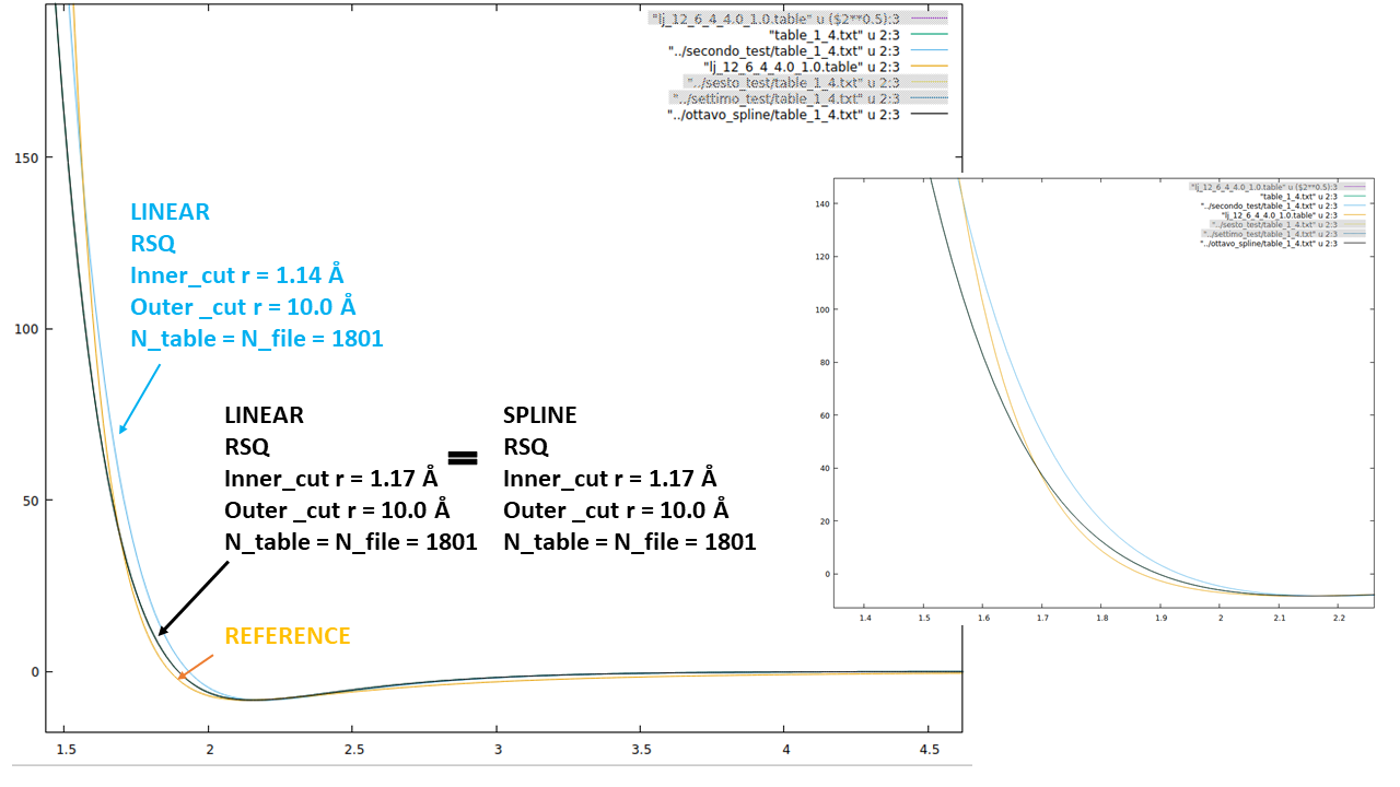
I tried to print the preliminary spline interpolation elaborated by LAMMPS, using the linear style, Ntable = Nfile and I tried both the R and the RSQ style. In my tabulated potential I considered the potential and the force at all distances between 1.0 Å and 10.0 Å to avoid fitting in the steepest region of the LJ repulsive branch and to use the same outer cutoff as the one used for the other pair_style respectively. I attach the lines of the test using RSQ style just as an example:

pair_style hybrid/overlay lj/cut/coul/long 10.0 10.0 coul/long 10.0 table linear 1801 ewald
pair_modify mix geometric
pair_modify tail yes
special_bonds lj/coul 0.0 0.0 0.5

kspace_style ewald 0.0001
include “pair_coeff.txt”

where pair_coeff.txt includes lines such as
pair_coeff 1 4 coul/long
pair_coeff 1 4 table lj_12_6_4.table POTENTIAL__1_4
pair_write 1 4 1801 rsq 1.0 10.0 table_1_4.txt POTENTIAL__1_4

The POTENTIAL__1_4 section of lj_12_6_4.table (my tabulated LJ) is the following

# DATE: 2022-25-10 UNITS: real CONTRIBUTOR: Emma (header line)
#12_6_4 potential for Zn (one or more comment or blank lines)

POTENTIAL__1_4
N 1801 RSQ 1.0 10.0

1 1.00 41531.50 503487.00
2 1.06 30056.62 355471.42
3 1.11 22103.39 255441.13
4 1.17 16490.52 186509.33
[…]
118 7.44 -4.38 -4.08
119 7.49 -4.32 -4.05
120 7.55 -4.26 -4.01
[…]
1800 99.95 -0.03 -0.01
1801 100.01 -0.03 -0.01

Increasing the distance, the potential has a minimum as expected from a LJ potential.
However, the file generated by LAMMPS is

# Pair potential hybrid/overlay for atom types 1 4: i,r,energy,force

POTENTIAL__1_4
N 1801 RSQ 1 10

1 1 83774.7220705805 1006396.11241192
2 1.02713192920871 60784.833626375 710594.257489771
3 1.05356537528527 44842.4797601862 510701.361776132
4 1.07935165724615 33584.5343687146 372962.001222688
[…]
118 2.7267196408872 76.1345668269373 68.8347968944961
119 2.7367864366808 75.4641403223875 68.1541852804469
120 2.74681633896407 74.8034404977079 67.4954486143175
[…]
1800 9.99724962177098 0.00431673939449543 0.0255875076741771
1801 10 0 0

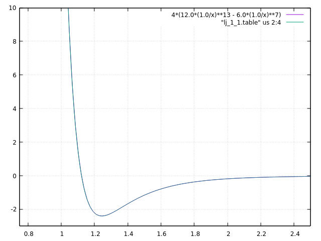
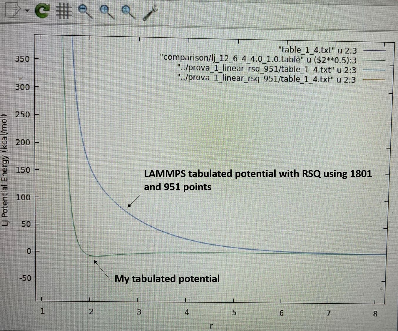
I plotted the two potentials they look completely different (as it emerges from the values in the tables). The most worrying difference is that the LAMMPS potential has no minimum and never goes to negative values. As I said, I also tried using R instead of RSQ, I reduced the points (951), but LAMMPS generates exacly the same curve. I attach a graph.

I cannot figure out what is the error I made in my input files since the RSQ of my table and the R of the LAMMPS table are consistent. I would be enormously grateful if someone could help me.

Thank you very much in advance for your kind collaboration.

Best regards,
Emma Rossi

One is only the LJ potential, the other is LJ plus coulomb due to using hybrid/overlay.

If you want to compare, I suggest you comment out the coul/long contribution and the kspace style.

In general, for testing/debugging your input, I strongly recommend to produce specific inputs that allow you to check individual components and not your project specific (final) input (and system).

Please also note the difference in your input table that seems like a linear tabulation with just outputting squared distances and not a tabulation with spacing that grows for large r.

Dear Axel,
thank you for your prompt reply. I am trying to implement your suggestions.

I have generated the simplest model I can to debug the input. The system contains only water molecules (TIP3P) and one Zinc ion. However, I still have to use the pair_style hybrid since water-water interactions are described through a Coulomb + 12-6 Lennard Jones potential, while Zinc-water interactions are regulated by the Coulomb + 12-6-4 LJ. I removed the coulombic part from Zinc-water interactions as well as ewald from the pair_style command line, as you suggested, to look at just LJ 12-6-4.

Now my input is
pair_style hybrid lj/cut/coul/long 10.0 10.0 table linear 1801
pair_modify mix geometric
pair_modify tail yes
special_bonds lj/coul 0.0 0.0 0.5 #not applied in this simple model
*kspace_style ewald 0.0001 *
include “pair_coeff.txt”

and pair_coeff.txt is

pair_coeff 1 1 lj/cut/coul/long 0.15210 3.15062 #WATER-WATER
[…]
pair_coeff 2 4 table lj_12_6_4.table POTENTIAL__2_4 #ZINC-WATER
pair_write 2 4 1801 rsq 1.0 10.0 table_2_4.txt POTENTIAL__2_4
pair_coeff 3 4 table lj_12_6_4.table POTENTIAL__3_4
pair_write 3 4 1801 rsq 1.0 10.0 table_3_4.txt POTENTIAL__3_4
pair_coeff 1 4 table lj_12_6_4.table POTENTIAL__1_4
pair_write 1 4 1801 rsq 1.0 10.0 table_1_4.txt POTENTIAL__1_4

Concerning the input table, I probably misunderstood the manual " for “RSQ”, squared distances uniformly spaced between rlorlo* and rhirhi* are computed." (pair_style table command — LAMMPS documentation) Could you please confirm that now I have understood correctly?
You mean that, for example, for a range of r 0-10 Å (0,1,2,3, etc…), I should write:

N the number of lines RSQ 0 10.0
RSQ Epot Force
0 Epot for r=0 Force for r=0
1 Epot for r=1 Force for r=1
4 Epot for r=4 Force for r=4
9 etc … etc …
16 etc… etc …

In such a way the spacing between consecutive points increases. Am I right?

Thank you in advance for the support and the patience.
Best regards,
Emma Rossi

To check out a potential and double check the tabulation, you do not need to build a realistic system. You don’t even need any atoms in it. Just create an empty box with one atom type, set the pair style and pair coeff and then you can use pair_write.

The easiest way to learn what different tables with different settings for a given potential look like, is to follow the same strategy as explained above, but use an analytic pair style like lj/cut or morse and then use the pair_write command with the different settings. That will show you what LAMMPS expects.

Dear Axel,
Thank you for your suggestions. I worked on them and the following is the best result I obtained. Using table, RSQ, and N table = N file as suggested in the documentation, I kept fixed the outer cutoff and I increased the inner cutoff. This led to better results in reproducing the potential well, but deviations from the reference still are present, in particular concerning the repulsive branch of Lennard Jones potential. Even greater inner cutoffs produce worse potentials and increasing the number of points does not lead to improvements. I tried also with spline style, but, as you can see from the graph, nothing changed.

Do you have any suggestions to improve my fitting? Or do you think, in your personal experience with pair_style table, that this fitting is already satisfactory? Thank you very much for your help.

Best regards,
Emma Rossi

There is no information, no LAMMPS inputs describing how you got the data.
Also, I don’t see any 12-6 potential tables that are easily compared to the analytic 12-6 potential. Without information on how the data is obtained and specifically a proper comparison to an analytic potential, there is no suggestion I can make. The difference you see is far beyond what would be the result of tabulation, so I suspect that you are (still) not comparing the same data.

As an illustration, attached is a plot comparing the analytical 12-6 LJ potential in reduced units with a tabulation generated by the following LAMMPS input:

region          box block 0 1 0 1 0 1
create_box      1 box
mass            * 1.0
pair_style     lj/cut 2.5
pair_coeff     * * 1.0 1.0
pair_write      1 1 2000 rsq 0.01 2.5 lj_1_1.table LJ

It is hard to see, but the two plots are virtually identical.
lj_12_6

Same for the force:
lj_12_6_force

1 Like

Dear Axel,
the table I generated was uncorrect, as you were guessing. I understood how to provide tabulated data in the correct way and, now, LAMMPS fitted potential are completely superimposable to mine.

Thank you very much for your support.
Best regards,
Emma Rossi