Dear Dynasor developers,
I’m using Dynasor to analyze LAMMPS MD trajectories of a 2D GaN monolayer and I’d appreciate your advice on whether I’m setting up the calculations correctly.
My setup is: (a) System: 2D GaN monolayer with vacuum in the out-of-plane direction, (b) T = 300 K, (c) Trajectory: 10000 frames from a NVE run, (d) Atoms: 12800 in total, 6400 Ga and 6400 N-atoms, and (e) Input to Dynasor: LAMMPS dump file with the full trajectory.
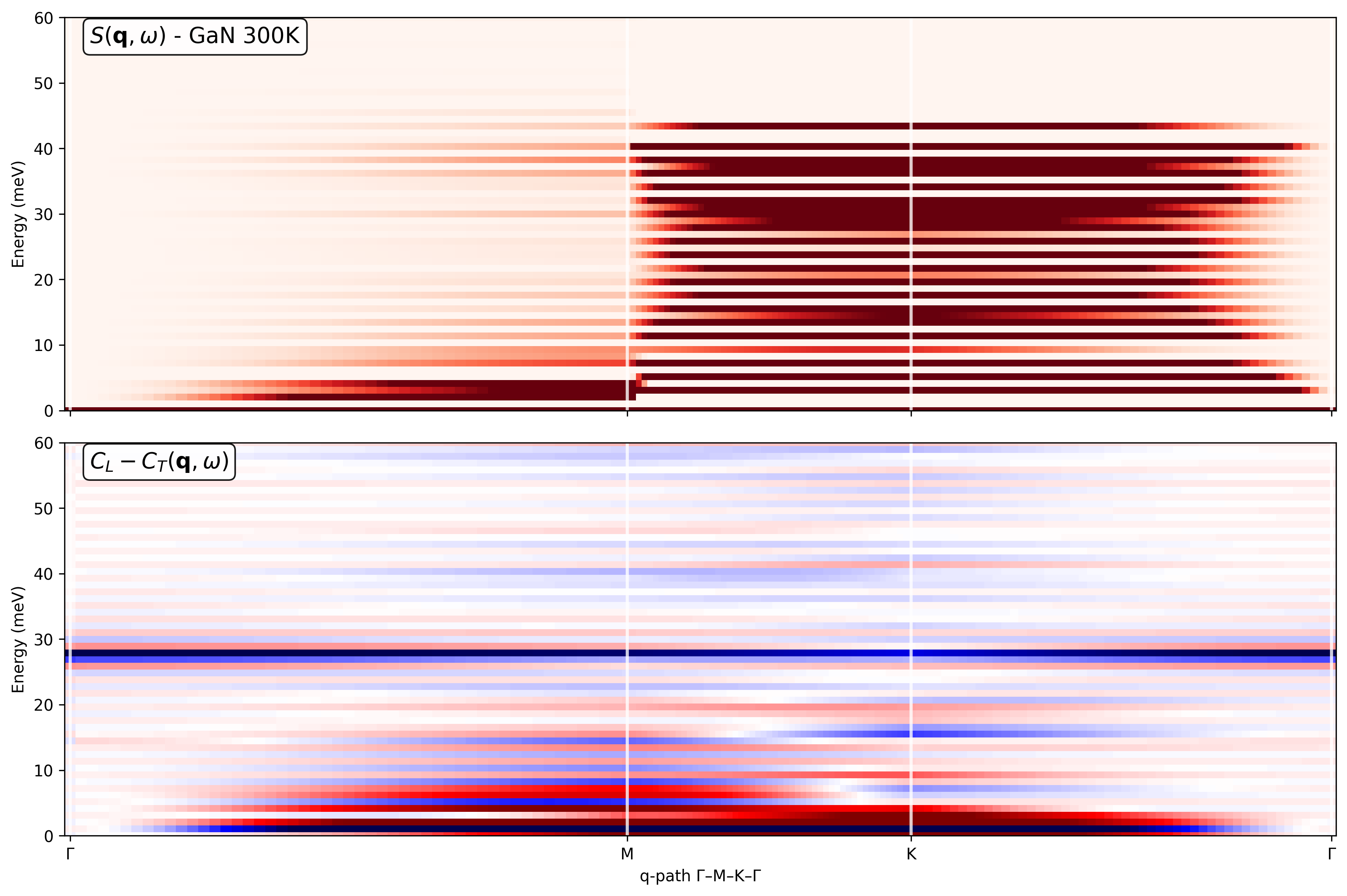
My goal is to obtain: (a) Phonon-like dispersions S(q,w) along a high-symmetry in-plane path (Gamma-M-K-Gamma) for the 2D Brillouin zone and (b) Partial current correlations and dynamical structure factors resolved into Ga-Ga, Ga-N, and N-N contributions.
I construct the q-path using the simulation cell, and I try to separate Ga and N using atomic_indices so that I can access the fields Sqw_Ga_Ga, Sqw_Ga_N, Sqw_N_N, Sqw_total, Clqw_Ga-Ga, Clqw_Ga-N, Clqw_N-N, Clqw_total, Ctqw_Ga-Ga, Ctqw_Ga-N, Ctqw_N-N, Ctqw_total, etc. I then generate the partial current correlations maps.
However, I’m unsure whether the resulting partial currents are physically meaningful.
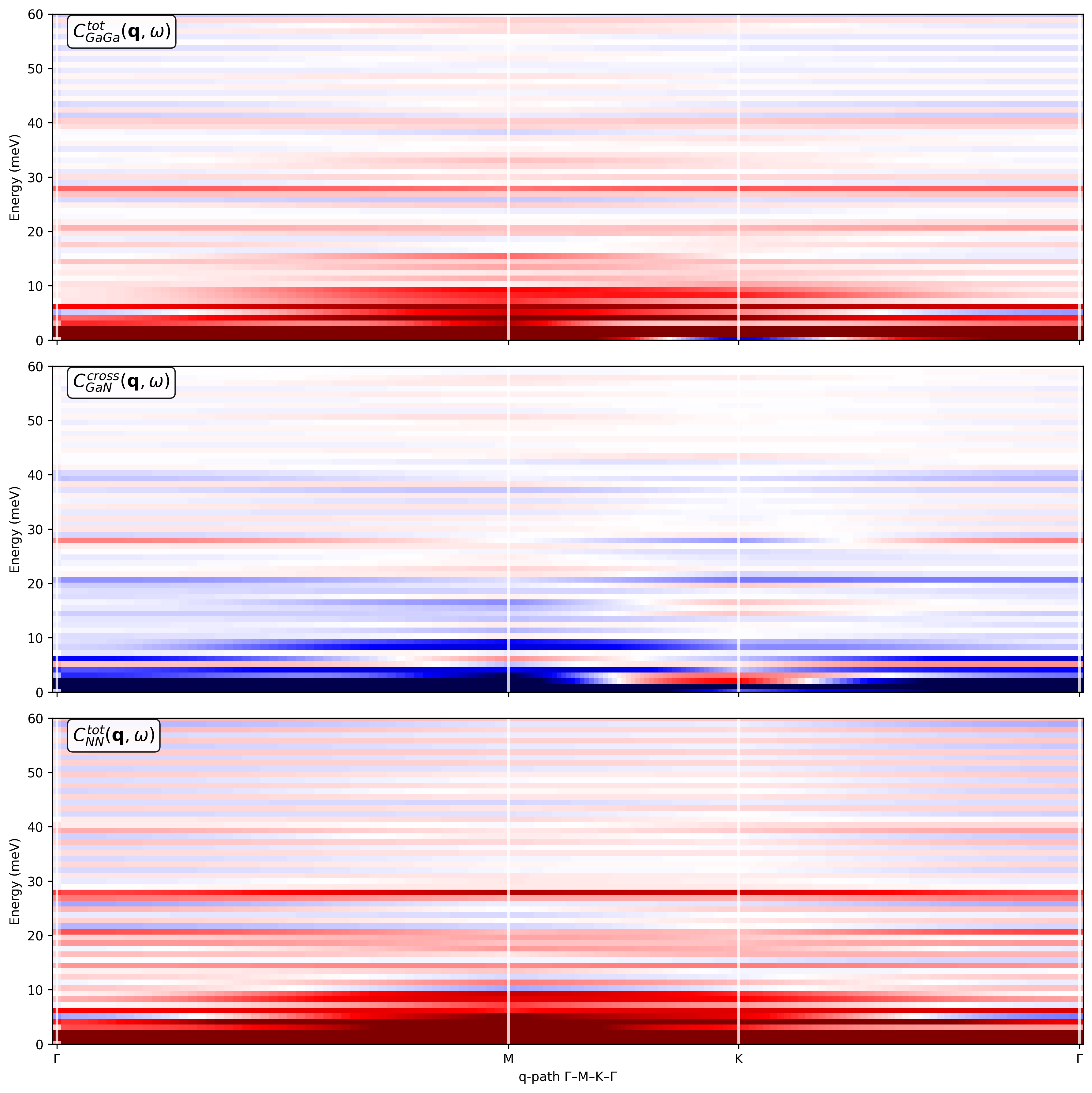
I’m attaching: (a) The Python code used to compute the dynamical structure factors and current correlations and (b) The resulting plots are at 300 K, including the Ga-Ga, Ga-N, and N-N partial current correlations.
Could you please let me know: (a) Whether my general approach is correct for a 2D monolayer treated as a 3D cell with vacuum and (b) Any obvious issues you can spot in the attached code or plots that might explain suspicious features in the partial current correlations.
Any guidance or example scripts for a binary 2D system (similar to GaN) would be extremely helpful. I’d also be happy to provide the trajectory if that would assist in diagnosing the problem.
Thank you very much for your time and for developing Dynasor. Looking forward to hearing from you.
Best Regards
Bishwajit Debnath
Research Scholar
Dept. of Chemistry
School of Physical Sciences
Sikkim University, Gangtok
India-737102
Email- [email protected]
"import numpy as np
from ase.io import read
from matplotlib import pyplot as plt
from dynasor import compute_dynamic_structure_factors, Trajectory
from dynasor.units import radians_per_fs_to_meV
------------------ Load trajectory ------------------
traj = Trajectory(‘gan_dump.lammpstrj’,
trajectory_format=‘lammps_internal’,
length_unit=‘Angstrom’,
time_unit=‘fs’,
frame_step=1,
frame_stop=10000)
print(traj)
Just to see the real cell
structure = read(‘gan_dump.lammpstrj’, index=0, format=‘lammps-dump-text’)
print(“Real cell dimensions:”, structure.cell.diagonal())
------------------ Species mapping Ga / N ------------------
n_atoms = traj.n_atoms
n_ga = n_atoms // 2
atomic_indices = {
‘Ga’: list(range(n_ga)),
‘N’: list(range(n_ga, n_atoms))
}
print(“Ga atoms:”, len(atomic_indices[‘Ga’]))
print(“N atoms:”, len(atomic_indices[‘N’]))
Reload trajectory with species separation
traj = Trajectory(‘gan_dump.lammpstrj’,
trajectory_format=‘lammps_internal’,
atomic_indices=atomic_indices,
length_unit=‘Angstrom’,
time_unit=‘fs’,
frame_step=1,
frame_stop=10000)
print(traj)
------------------ q-path Γ–M–K–Γ in ABSOLUTE q (rad/Å) ------------------
Simulation cell (Å)
A = np.array(traj.cell) # shape (3,3)
Reciprocal lattice (rad/Å), columns are b1,b2,b3
B = 2.0 * np.pi * np.linalg.inv(A).T # dynasor expects 2π included
High-symmetry points in reduced (fractional) coordinates
Gamma_frac = np.array([0.0, 0.0, 0.0])
M_frac = np.array([0.5, 0.0, 0.0])
K_frac = np.array([1/3., 1/3., 0.0])
Convert to absolute Cartesian q: q_abs = B @ q_frac (rad/Å)
Gamma_q = B @ Gamma_frac
M_q = B @ M_frac
K_q = B @ K_frac
def segment(q_start, q_end, npts):
return np.linspace(q_start, q_end, npts, endpoint=False)
n_points_per_segment = 50
q_GM = segment(Gamma_q, M_q, n_points_per_segment)
q_MK = segment(M_q, K_q, n_points_per_segment)
q_KG = segment(K_q, Gamma_q, n_points_per_segment)
q_points = np.vstack([q_GM, q_MK, q_KG]) # (150, 3)
enforce in-plane qz = 0 (monolayer)
q_points[:, 2] = 0.0
print(f"Generated {len(q_points)} ABSOLUTE q-points along Γ–M–K–Γ path")
------------------ Dynamic structure factors ------------------
sample = compute_dynamic_structure_factors(traj, q_points,
dt=1.0,
window_size=2000,
window_step=100,
calculate_currents=True)
sample.omega *= radians_per_fs_to_meV
print(sample)
------------------ q-distance along path ------------------
cumulative distance along the ABSOLUTE q-points
dq = np.linalg.norm(np.diff(q_points, axis=0), axis=1)
q_distances = np.concatenate([[0.0], np.cumsum(dq)]) # len = len(q_points)
idx_G = 0
idx_M = n_points_per_segment
idx_K = 2 * n_points_per_segment
idx_G2 = len(q_points) - 1
q_labels_pos = [idx_G, idx_M, idx_K, idx_G2]
q_labels = [‘Γ’, ‘M’, ‘K’, ‘Γ’]
------------------ Plot 1: S(q,ω) and C_L - C_T ------------------
fig, (ax1, ax2) = plt.subplots(2, 1, figsize=(12, 8), sharex=True, dpi=150)
S(q,ω)
im1 = ax1.pcolormesh(q_distances, sample.omega, sample.Sqw_coh.T,
cmap=‘Reds’, vmin=0, vmax=8)
ax1.text(0.02, 0.98, r’S(\mathbf{q}, \omega) - GaN 300K’,
transform=ax1.transAxes, va=‘top’, fontsize=14,
bbox=dict(boxstyle=“round,pad=0.3”, facecolor=“white”, alpha=0.9))
ax1.set_ylabel(‘Energy (meV)’)
ax1.set_ylim(0, 60)
C_L - C_T
m_lt = 0.1 * np.max(np.abs(sample.Clqw.T - sample.Ctqw.T))
im2 = ax2.pcolormesh(q_distances, sample.omega,
sample.Clqw.T - sample.Ctqw.T,
cmap=‘seismic’, vmin=-m_lt, vmax=m_lt)
ax2.text(0.02, 0.98, r’C_L - C_T(\mathbf{q}, \omega)‘,
transform=ax2.transAxes, va=‘top’, fontsize=14,
bbox=dict(boxstyle=“round,pad=0.3”, facecolor=“white”, alpha=0.9))
ax2.set_ylabel(‘Energy (meV)’)
ax2.set_xlabel(r’q-path Γ–M–K–Γ’)
ax2.set_ylim(0, 60)
for ax in [ax1, ax2]:
for pos in q_labels_pos:
ax.axvline(q_distances[pos], c=‘white’, lw=2, alpha=0.8)
ax2.set_xticks([q_distances[i] for i in q_labels_pos])
ax2.set_xticklabels(q_labels)
plt.tight_layout()
plt.savefig(‘GaN_Sqw_Clt.png’, dpi=300, bbox_inches=‘tight’)
plt.show()
------------------ Plot 2: Ga–Ga, Ga–N, N–N currents ------------------
fig, axes = plt.subplots(3, 1, figsize=(12, 12), sharex=True, dpi=150)
Ga–Ga
m_gg = 0.1 * np.max(np.abs(sample.Clqw_Ga_Ga.T + sample.Ctqw_Ga_Ga.T))
axes[0].pcolormesh(q_distances, sample.omega,
sample.Clqw_Ga_Ga.T + sample.Ctqw_Ga_Ga.T,
cmap=‘seismic’, vmin=-m_gg, vmax=m_gg)
axes[0].text(0.02, 0.98, r’C_{GaGa}^{tot}(\mathbf{q}, \omega)',
transform=axes[0].transAxes, va=‘top’, fontsize=14,
bbox=dict(boxstyle=“round,pad=0.3”, facecolor=“white”, alpha=0.9))
axes[0].set_ylabel(‘Energy (meV)’)
axes[0].set_ylim(0, 60)
Ga–N
m_gn = 0.1 * np.max(np.abs(sample.Clqw_Ga_N.T + sample.Ctqw_Ga_N.T))
axes[1].pcolormesh(q_distances, sample.omega,
sample.Clqw_Ga_N.T + sample.Ctqw_Ga_N.T,
cmap=‘seismic’, vmin=-m_gn, vmax=m_gn)
axes[1].text(0.02, 0.98, r’C_{GaN}^{cross}(\mathbf{q}, \omega)',
transform=axes[1].transAxes, va=‘top’, fontsize=14,
bbox=dict(boxstyle=“round,pad=0.3”, facecolor=“white”, alpha=0.9))
axes[1].set_ylabel(‘Energy (meV)’)
axes[1].set_ylim(0, 60)
N–N
m_nn = 0.1 * np.max(np.abs(sample.Clqw_N_N.T + sample.Ctqw_N_N.T))
axes[2].pcolormesh(q_distances, sample.omega,
sample.Clqw_N_N.T + sample.Ctqw_N_N.T,
cmap=‘seismic’, vmin=-m_nn, vmax=m_nn)
axes[2].text(0.02, 0.98, r’C_{NN}^{tot}(\mathbf{q}, \omega)‘,
transform=axes[2].transAxes, va=‘top’, fontsize=14,
bbox=dict(boxstyle=“round,pad=0.3”, facecolor=“white”, alpha=0.9))
axes[2].set_ylabel(‘Energy (meV)’)
axes[2].set_xlabel(r’q-path Γ–M–K–Γ’)
axes[2].set_ylim(0, 60)
for ax in axes:
for pos in q_labels_pos:
ax.axvline(q_distances[pos], c=‘white’, lw=2, alpha=0.8)
axes[2].set_xticks([q_distances[i] for i in q_labels_pos])
axes[2].set_xticklabels(q_labels)
plt.tight_layout()
plt.savefig(‘GaN_partial_currents.png’, dpi=300, bbox_inches=‘tight’)
plt.show()
print(“GaN phonon dispersion ALONG Γ–M–K–Γ PATH COMPLETE!”)
print(f"Supercell: {traj.cell.diagonal()}“)
print(f"Ga: {len(atomic_indices[‘Ga’])} atoms, N: {len(atomic_indices[‘N’])} atoms”)"