shock propagation through bulk system

Dear all,
I am trying to set up a model and doing NEMD to study shock propagation through single crystal. In this context I have gone through all the previous discussions regarding this from lammps archive. Firstly i’m using fs b/c along shock direction and then generating shock by using wall/reflect and velocity setting, i.e “momentum mirror” method. Here i’m pasting some of the part of my script –

pressure_shockdirection.png

temperature_shock_direction.png

Hi Vishnu,

The temperature is increasing: it has increased from ~500K to ~1000K
behind the shock wave. There is some smearing but is still increasing
due to shock compression. More comments below.

Ray

velocity all set 3.0 0.0 0.0 sum yes units box

Unless you are changing signs elsewhere not shown, your sample is
going towards the right.

The script ran fine but I need some justification about some issues which is
not clear to me,
the first observation is, i'm getting P-T curve of the shocked sample and
it's showing that temperature is decreasing when pressure is increasing (i
have attached the plot). When the existing literature suggests that

T is indeed increasing.

temperature should increase with pressure and as the matter of fact it
should show some kink at a significant pressure. I am seeing that as soon as
simulation is getting started the nearer atoms of the left mirror showing
the velocity less than the velocity, I set to every atoms towards the left
mirror(i.e the left most lair of system). Is this the cause i.e why

It seems your sample is right next to the wall with no space in
between, and this is probably the reason you are seeing an instant
increase in velocities.

temperature is falling down behind shock front ? I am attaching
temperature and pressure variation along the shock direction for your
convenience.

The another question is that in classical MD we are not taking the
electronic contribution to compute temperature, so how this temperature
would be justified or would be comparable with macroscopic/experimental
results specially for NEMD and shock like high temperature phenomenon ?

You are not going to get any electronic contribution since this is
purely atomic. Presumably the electron-electron and electron-core
interactions are all included in the core-core interaction during the
fitting of the EAM potential.

Dear Shan,
it was a mistake while I was pasting my script, I am furnishing the full script here…please see, BTW regarding electronic contribution of temperature, you are quite correct but to get such high temperature been possible for shock experiment ? I mean at 10000 K copper copper should be in vapor state, how can I justify this. I have gone through a lots of literature but most of them are not mentioning the temperature.

NEMD Shock experiment with a copper bulk

System dimensiion 400100100 unit cells in X,Y and Z direction

Method: Single Impact Shock

Potential: EAM cu Foiels et al

#-----------------------Initialization-------------------------------------#
variable kB equal 1.3806504e-23 # [J/K] Boltzmann
variable Na equal 6.02e23 # Avogardo number
variable pconv equal 0.0001 # bar to GPa
variable vconv equal 0.100 # A/ps to Km/sec
variable wallleft equal -8.05858552526837698e-03 # in length unit
variable wallright equal 1.4462248969819657e+03 # in length unit
variable SHOCKVEL equal 1.5 # km/s
variable Init_Vol equal 10455.6233191.0e-24 # Cm3
variable Init_Leng equal 144.614430415 # in Angstrom
variable vel equal ${SHOCKVEL}
-10 # A/ps

#-----------------------System Variable Initialization ---------------------#

units metal
atom_style atomic
boundary fs p p

#-----------------------System Description from data file ------------------#

read_data final_data

#-----------------------Force Field Setting --------------------------------#

pair_style eam
pair_coeff * * Cu_u3.eam
timestep .0005 # 0.5 fs, as in metal unit time is in ps. 1ps = 1000fs

#----------------------To compute spatialy averaged temperature profile --------#

velocity all set {vel} 0.0 0.0 sum yes units box fix 1 all nve fix 2 all wall/reflect xlo {wallleft} xhi ${wallright} units box

compute ke all ke/atom
variable temp atom c_ke/(1.5*8.61e-5)
fix temp_profile all ave/spatial 25 8 200 x lower 3.0 v_temp file temp.profile units box

#---------------------To compute spatialy averaged stress tensor averaged diagonal elements--------#

compute peratom all stress/atom
variable meanpress atom -(c_peratom[1]+c_peratom[2]+c_peratom[3])/3
fix pressure_profile all ave/spatial 25 8 200 x lower 3.0 v_meanpress units box file pressure.profile

#----------------To compute x comp of velocity in spatialy averaged method--------------------#

compute vx all property/atom vx
fix velX_profile all ave/spatial 25 8 200 x lower 3.0 c_vx units box file velocityXcomp.profile

#----------------To compute spatialy averaged density------------------------------------------#

fix densityX_profile all ave/spatial 25 8 200 x lower 3 density/number density/mass file densityX.profile units box
fix densityY_profile all ave/spatial 25 8 200 y lower 3 density/number density/mass file densityY.profile units box
fix densityZ_profile all ave/spatial 25 8 200 z lower 3 density/number density/mass file densityZ.profile units box

#---------------To compute spatialy averaged atomic displacement-----------------------------------#

compute disp_per_atom all displace/atom
variable dis atom c_disp_per_atom[4]
fix dis_profile all ave/spatial 25 8 200 x lower 3.0 v_dis file dis.profile units box

#----------------To compute time average of global pressure ----------------------------------------#

variable mypress equal press
fix mypressure all ave/time 25 8 200 v_mypress file global_pressure.profile

#----------------To compute time average of global temperature --------------------------------------#

variable mytemp equal temp
fix mytemperature_profile all ave/time 25 8 200 v_mytemp file global_temperature.profile

#----------------To compute time average of kinetic energy ------------------------------------------#

variable myke equal ke
fix myke_profile all ave/time 25 8 200 v_myke file global_mykineng.profile

#---------------- To compute time average volume -----------------------------------------------------#

variable myvol equal vol
fix myvol_profile all ave/time 25 8 200 v_myvol file global_volume.profile

#---------------- To dump the trajectory -------------------------------------------------------------#

dump 1 all custom 1000 *.cfg id type xs ys zs id vx vy vz fx fy fz
dump_modify 1 element Cu

#------------------ thermo output ----------------------------------------------------------------------#
thermo 1000
thermo_style custom step temp pe ke etotal press vol lx xlo xhi
thermo_modify norm yes

#-------------------- Setting up of shock technicque-----------------------------------------------------#
restart 5000 *.restart

run 20000

write_restart restart.final

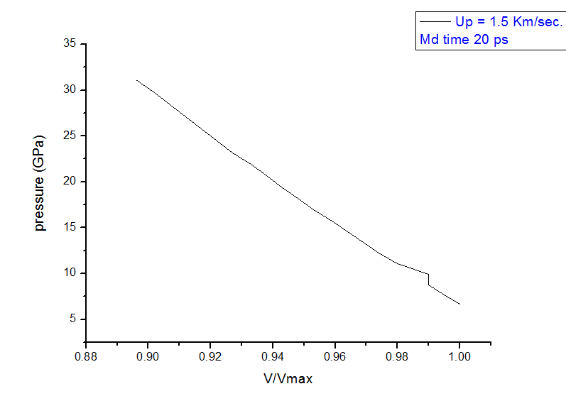
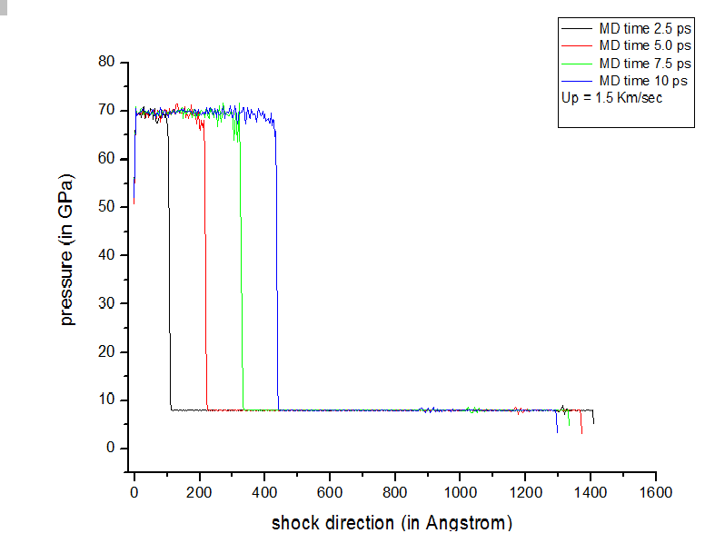
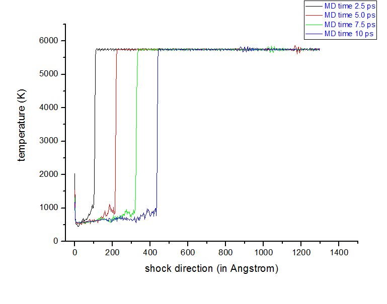
here I am setting the velocity along -X direction so, surely shock should propagate towards +X. So my plots showing that not BEHIND the shock, temp is increasing and pressure is decreasing, in-front the shock front. Behind the shock front temperature is decreasing and pressure is increasing, which is quit wrong. There is something which I am missing, please correct me.
I am attaching more plots to clear the fact more clear.

thanks

pressure_volume_fraction.png

Vishnu,

No, you are not considering the center-of-mass translational velocity
that contributed to your temperature calculations (so-called "flying
ice cube" problem). The ~5600K temperature that you think is high
actually includes the SHOCKVEL you assigned and added (through
velocity sum yes) to the sample - which is bogus and means nothing
physical at all. The actual temperature of the whole sample is ~500K.

To make it clear: In your plot, temperature of uncompressed sample
that is still moving towards the wall *means nothing*, and temperature
of compressed materials behind the shock front has increased from
~500K to ~900K.

Hope this clear and helps.

Ray

Dear Shan,

yes, yes now it’s clear to me, thanks a lot for that. would it be correct if I calculate the temperature of the unshocked region by compute temp/deform command ?

you mention that there is no spacing in between wall and sample causing instantaneous increasing in velocity. So can i introduce that spacing by setting the left wall at -2 where the left edge of my sample is in -.008, i.e by doing this

fix 2 all wall/reflect xlo -2 xhi ${xrightwall} units box

In NEMD to study a long time evolution along shock is there any option excluding the way of increasing the system length along shock ? I mean like absorbing boundary condition ( which is not in lammps ).

Another things is that if I look at the pressure curve in shocked region, there is no significant rising in pressure, is it so ?

thanks

regards,

Vishnu

Vishnu,

For long-term shock trajectories there is either the hugoniostat method, or else ‘matched pistons’. For this latter option, generate your shock using a piston (rather than a momentum mirror) and create another group at the far end of the simulation. When the shock reaches that point, set the motion of the second piston to match that of the first (shock generating) piston.

Nigel

Hi,

I’m just reading this post (not commenting) , since Ray and Nigel already gave valuable comments and i don’t know what else I could say. Anyways i just wanted to thank you guys for this valuable feedback … =)

PS: I believe Ab-initio molecular dynamics it’s being used use to model Shock phenomena thus electron-interaction its counted. Althought I havent tried to run this kind of simulations because they are way too expensive for my current PC power

A salute
Oscar G.

Hi Nigel

thanks for your feedback, I have seen several papers on Hugoniostat method to track long term shock trajectories, but can you please refereed me a literature for the second method you mention, ‘matched pistons’.

Thanks for your time.

Hi Shan,

thanks for your suggestion, you say well “temp/com” should be the appropriate solution. BTW to take care of the space in-between piston and sample, I am modifying my data file as (xlo + 2 ) and (xhi - 2 ), keeping y and z values unchanged, and also setting my piston at xlo and xhi. Would it be correct to consider the space ?

thank you

rgds,

Vishnu

thanks for your suggestion, you say well "temp/com" should be the
appropriate solution. BTW to take care of the space in-between piston and
sample, I am modifying my data file as (xlo + 2 ) and (xhi - 2 ), keeping y
and z values unchanged, and also setting my piston at xlo and xhi. Would it
be correct to consider the space ?

You should be able to just use change_box command to increase xhi,
then displace your sample +2.0 in x.

Ray

http://www.dtic.mil/dtic/tr/fulltext/u2/a521064.pdf

Dear Shan,

really sorry for such beginner level question, but plz

by using chenge_box ( change_box all x final 0 1402 boundary p p p units box ) I am now shifting my xhi from 1400 to 1402 keeping y, z and volume preserve, but now how can I displace my sample +2 towards x, is this by displace_atom or anything else ?

thanks

Vishnu

Hi Ray,
I have seen that “displace_atoms” command with style “move” in a specific dirn can move the simulation domain to a desired 3d direction before simulation, so if I have not missing anything, the following modification can solve my problem, if any wrong plz correct it…

variable wallleft equal 0
variable wallright equal 1400

change_box all x final 0 1402 boundary fs p p units box
displace_atoms all move 2 0 0 units box
fix 2 all wall/reflect xlo {wallleft} xhi {wallright} units box

Hi,

This reference its really explanatory and it helped me to understand how to track the position of the shock front by monitoring the time dependence of the center-of-mass (COM). Hopefuly it may be useful.

REF: Molecular dynamics simulations of shock waves in oriented nitromethane single crystals http://dx.doi.org/10.1063/1.3561397

PS: right now i’m looking at Vishnut Script , and trying to understand it, but brain is out of power, and i’m watching Cartoons via YouTube…

A salute
Oscar G.

1 Like