Simulating liquid-vapour coexistence of a Lennard-Jones fluid

Hi all,

As part of a bigger project I'm trying to establish the saturation pressure of a Lennard-Jones fluid, or, more specifically, the truncated and shifted Lennard-Jones potential (implemented in LAMMPS as lj/cut). It is well known in literature that quantitative thermodynamic properties depend on the truncation point of the potential [1], so I thought the most straightforward method to establish this for my system is to run some NVT simulations myself for different densities while outputting the pressure.

For a vapour in equilibrium with its liquid phase, the pressure should be constant and equal to the equilibrium vapour pressure (saturation pressure) of the fluid. So as long as I'm in the coexistence region, the pressure of my system should be independent of the overall density.

I found this NIST data with accompanying LAMMPS input script (very convenient) that basically does this [2]. The only difference is that they use the linear force-shifted LJ potential (formerly implemented as lj/sf, nowadays it's lj/smooth/linear) instead of lj/cut.

Now the problem: I can't manage to produce the constant pressure behaviour that I expect. Depending on my boundary conditions and potentials, the pressure of my system either increases or decreases with overall density. Neither are physically correct behaviour for such a system, to my understanding at least.

My findings are as follows:

With lj/cut (cut at 2.5 sigma) as potential, PBCs in xyz, I find that the pressure *decreases* with increasing density. At an overall density of 0.185 I have a pressure of ~0.02. When I double the density to 0.37, the pressure reads as ~0.007.

With the cut-off at 5 sigma, I managed to produce *negative* pressures at one point. I don't understand how this is possible for a Lennard-Jones fluid.

If I use the lj/smooth/linear potential like the NIST people do, the differences in pressure are smaller, but still not constant like I would expect:

density pressure
0.1 0.050
0.185 0.047
0.37 0.040

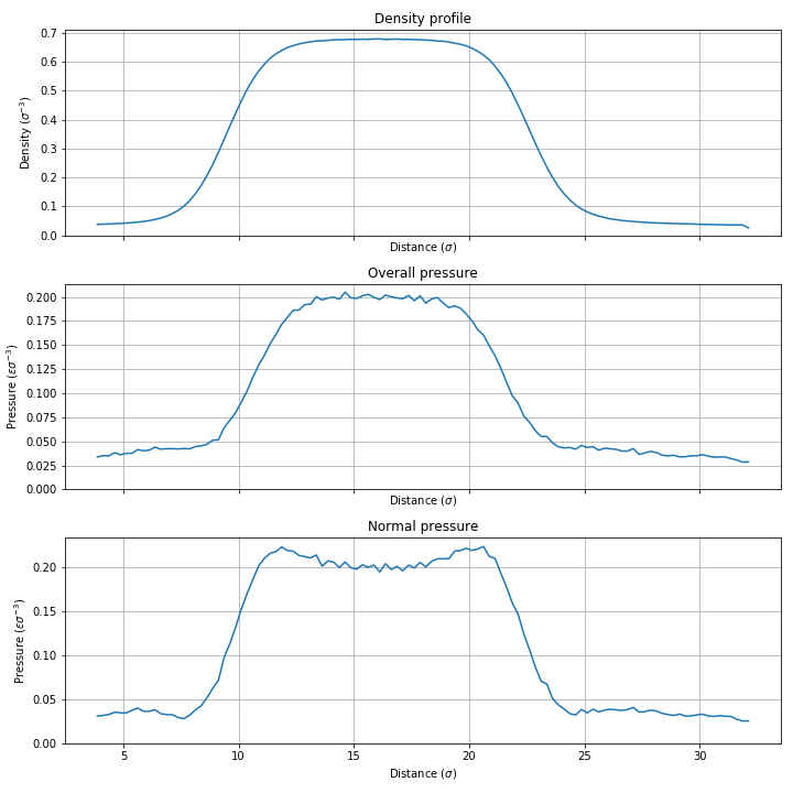
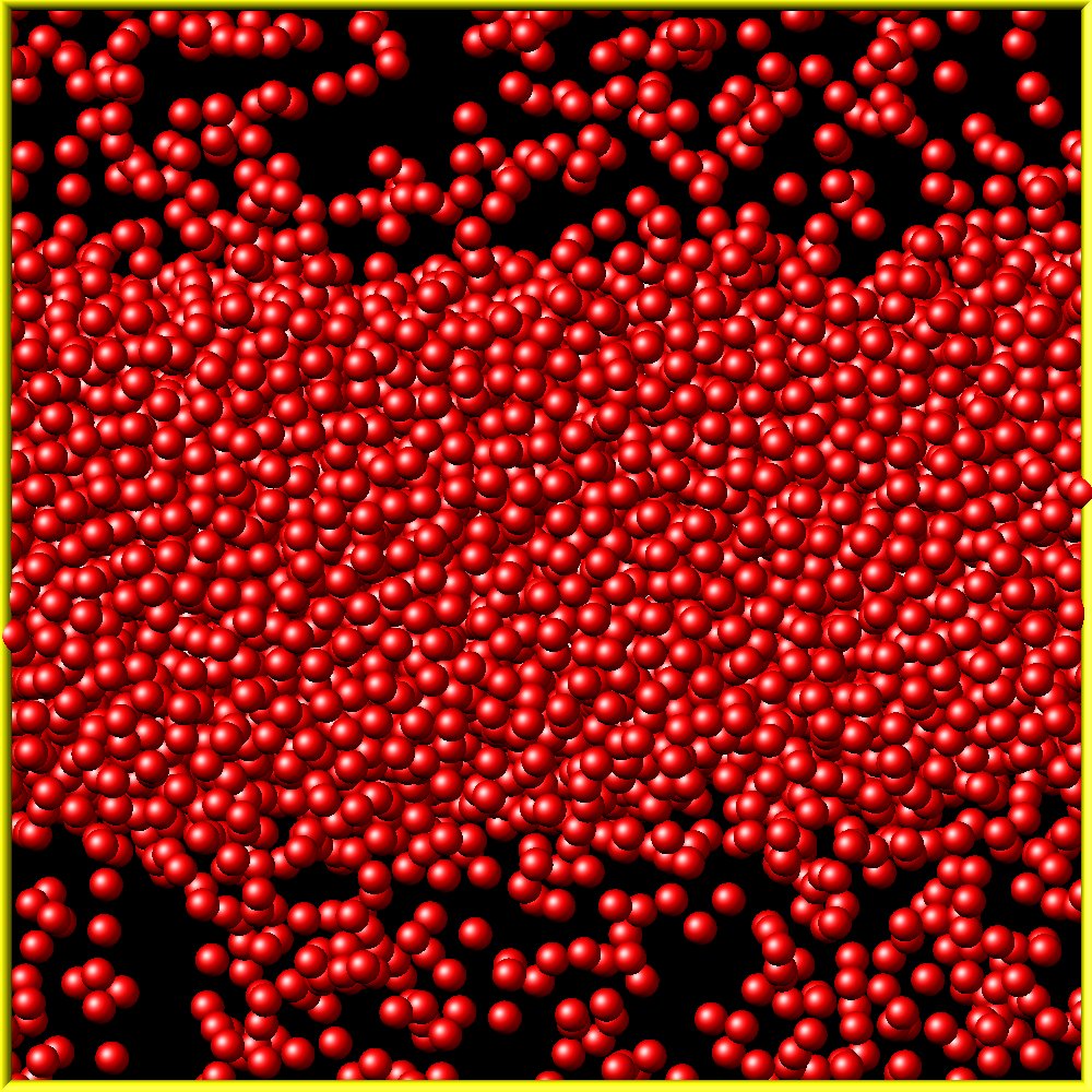
If I make one dimension (z) fixed and install a wall at the top and bottom of the box and add a small gravity force (0.01) to get layering (I did this so I can easily analyse the densities of the two phases separately), get *increasing* pressure with density:

density pressure
0.1 0.041
0.2 0.046
0.3 0.059

All simulations are performed at a temperature T=0.85 (subcritical, of course) and all numbers are in reduced LJ units.

At this point I don't really know what to make of this. Are my assumptions correct? Is the problem in the pressure calculation? Is this an artifact of the (truncated) Lennard-Jones potentials? Something else even?

Ideas are appreciated.

Lars Veldscholte

[1] Smit, B. Phase Diagrams of Lennardā€Jones Fluids. The Journal of Chemical Physics 1992, 96 (11), 8639ā€“8640. https://doi.org/10.1063/1.462271.

[2] https://www.nist.gov/mml/csd/informatics/lammps-md-equation-state-pressure-vs-density-linear-force-shifted-potential-25s

Well, Lennard-Jones is the most used potential so the issue is probably not there. Also I donā€™t think that, if there was an error in the pressure calculation, you would be the first to find it.
Why do you expect pressure to increase with increasing density? Are you perhaps confusing the total density of your simulation volume with the density of the liquid phase and the density of the gas phase?

Hi Stefan,

Thanks for your reply.

I don't expect the total pressure to increase with increasing density. Within the coexistence region, I expect the pressure to stay exactly constant with varying density, because I have a two-phase system (liquid in equilibrium with vapour). The density of the liquid phase and the density of the vapour phase should also stay constant of course, I only expect the distribution of liquid/vapour to shift. For example, if I increase the overall density of my system, I expect more liquid to condense, but the pressure to stay the same.

Lars

two questions come to my mind when reading this discussion:

  1. are you using the tail correction to the pressure for truncated potentials (pair_modify tail yes)?
  2. i assume the pressure data you quote are averages. have you discarded the equilibration parts of the simulation from this averaging and have you checked how well converged those averages are?

axel.

Iā€™m not using tail corrections. Should I be using it? The docs mention it should only be used for bulk homogeneous liquids, and not for two-phase systems like mine.

Thatā€™s correct, theyā€™re time-averaged values. I forgot to mention, but all simulations are run for 1M timesteps. Iā€™ve also looked at the time evolution of the pressure (and other thermo measures) and they are either already basically converged after the minimization, or converge quickly. So that is not the reason for inconsistency in pressure.

Lars

Iā€™m not using tail corrections. Should I be using it? The docs mention it should only be used for bulk homogeneous liquids, and not for two-phase systems like mine.

it is worth giving it a try to see, if you get more consistent results. since the LJ potential is always attractive beyond the cutoff, you are missing some contributions depending on the choice of cutoff. systematically increasing the cutoff would be another. the larger the cutoff the smaller the correction. :wink:
this is only a correction for the pressure so entirely diagnostic since you are running at fixed volume.

a more elaborate approach to include longer-range LJ contributions would be to use pair style lj/long/coul/long with ewald/disp or pppm/disp. if i remember correctly, you can disable the coulomb part of the computation (you may still need to use atom style charge, tough) and thus apply it to a pure LJ system.

axel.

Hi Stefan,

Thanks for your reply.

I donā€™t expect the total pressure to increase with increasing density.
Within the coexistence region, I expect the pressure to stay exactly
constant with varying density, because I have a two-phase system (liquid
in equilibrium with vapour).

I am bad at thinking in macroscopic quantities when it comes to thermodynamics. :slight_smile:

Total pressure remains the same because when you increase density, all particles that you add end up in the liquid phase?
So the density of the gas part is constant and hence the pressure is pretty much just the ideal gas pressure, i.e. density*kT?

The density of the liquid phase and the
density of the vapour phase should also stay constant of course

The liquid is almost completely incompressible and, if all extra particles end up in the liquid phase, then yes, I agree.

I only expect the distribution of liquid/vapour to shift. For example, if I
increase the overall density of my system, I expect more liquid to
condense, but the pressure to stay the same.

Right.

Tail corrections might help. 10000 particles is not small (not exactly huge but should be sufficient).

However, it might be good to take a step back and see if you can at least reproduce the NIST data?

Also, have you checked your simulation snapshots to make sure it looks like what you expect?

Thanks, Iā€™ll try that and report back.

Lars

Just a shot in the dark.
If you're taking the total system pressure, you're including the surface tension from your solid-liquid interface.
Be sure to only take the component perpendicular to the solid-liquid interface.
Either that, or maybe you have a droplet formed in your system.

Best regards,
Donatas

Indeed.

This is very well-trodden territory with a lot of prior detailed work that you can refer to. Also, I found nothing in your original description that was particularly surprising. Since you are moving along a subcritical isotherm from low density to high density, you should expect, at some point, to encounter the famous loop of your compatriot van der Waals. This contains a thermodynamically unstable interval of density where the pressure is decreasing, possibly even negative. Rather than assume there is something wrong with LAMMPS or your simulation, try reading a few papers of those who have gone before you. In fact, there is an excellent text book by two more of your compatriots, Frenkel and Smit, that covers this topic in great detail, including the subtle effects of discontinuities at the cutoff and tail corrections.

Aidan

Hi All,

I am now responding to the extra information provided in the follow-up responses. My original comments only apply to homogeneous, possibly metastable or unstable, phases. This is what you will tend to see if you run a small periodic system, where phase separation is supressed on MD timescales. This is also what is covered in Frenkel and Smitā€™s book. You mention that you are seeing two phases coexisting. That complicates matters greatly. The total pressure now contains large contributions from interfacial regions, and so will depend strongly on the morphology of the interfaces (liquid drops, liquid slabs, bicontinuous gas/liquid and so on). This is not well-trodden territory. You should expect to be surprised. If you are interested in saturation pressure, you will need to be much more careful about how you measure pressure. One strategy would be to first equilibrate a 2-phase slab system, then calculate local pressure (compute stress/atom) as a function of distance from the interface. You should see the same pressure in the middle of the vapor region and in the middle of the liquid region. That said, I think you will find it a lot easier to focus on small systems where phase separation is suppressed.

Aidan

I think using the average pressure, i.e. the average of the trace of the pressure tensor, is too simplistic for a liquid-vapor interface. For a planar liquid-vapor interface, the component of pressure normal to the interface will be constant throughout the interface according to the mechanical stability requirement. However, the tangential component will not be constant through the interface and the difference between normal and tangential pressures is related to the surface tension in the interface. The normal and tangential components will of course be equal in either of the bulk phases.

If you have a small enough system in which phase separation is prohibited but your density is somewhere between the liquid and vapor coexistence densities, then you will follow an S-shaped (van der Waals loop) pressure isotherm, NOT the constant pressure line. For example see https://en.wikipedia.org/wiki/Maxwell_construction and https://scholarsarchive.byu.edu/etd/3248/.

Stan

So to clarify, you can get the ā€œconstantā€ pressure value you are expecting from your two-phase simulations, but you have to ensure that you have a well-defined planar interface and only consider the component of pressure normal to the interface. You can average this component over time to get a better value. However if you have bubbles or not enough of both phases to get a nice, clean planar interface or are close to the critical point, it probably wonā€™t work as Aidan said.

Stan

Thanks for your insightful comments.

To also reply to your previous email, yes, of course Iā€™m aware of the van der Waals loop. Thatā€™s, in essence, of course, the reason why phase separation happens in the first place.

But indeed, in my simulations I see phase separation so I expect the pressure to follow the Maxwell construction, i.e., stay constant. I didnā€™t realise that simulating a two-phase system was so tricky. I thought the interfacial pressure would cancel out if you average over the entire system.

Are you referring to the book ā€œUnderstanding Molecular Simulationā€ by Frenkel and Smit? Thanks for the tip, Iā€™ll look into it.

Lars

I have an update:

I re-ran my simulations with output of both the pressure profile and the normal pressure profile in Z. I get layering of my two phases in Z (see attached dump image) and the interface is an XY-plane.

It appears that there is still something strange going on. The pressure in the bulk of each of the phases is not equal; the pressure is almost an order of magnitude larger in the bulk of the liquid compared to the vapour. Looking at the profile of the normal pressure, there is some deviation from the overall pressure at the interfaces, but the pressures in the bulk of the two phases is not equal. (see attached plots)

I used the following input file lines to produce the profiles:

# Output fixes/dumps
compute cc2 all chunk/atom bin/1d z 0.0 0.25
fix prof_dens all ave/chunk \{Nevery\} {Nrepeat} ${Nfreq} cc2 density/number file SolvDens.dat

# Pressure profile
compute atom_stress all stress/atom thermo_temp
compute atom_vol all voronoi/atom
variable atom_press atom -(c_atom_stress[1]+c_atom_stress[2]+c_atom_stress[3])/3/c_atom_vol[1]
variable atom_press_z atom -c_atom_stress[3]/c_atom_vol[1]

fix prof_press all ave/chunk \{Nevery\} {Nrepeat} \{Nfreq\} cc2 v\_atom\_press file Pressure\.dat fix prof\_press\_z all ave/chunk {Nevery} \{Nrepeat\} {Nfreq} cc2 v_atom_press_z file PressureZ.dat

Aidan mentioned that it would be easier to simulate small systems where phase separation is suppressed. How would I go about determining the saturation pressure using such a simulation?

Lars

profiles.png

1000000.jpg

It looks like you didn't normalize properly. I've had success with using compute stress/atom directly in fix ave/chunk to get the local pressure, no need to use compute voronoi/atom. In fact, no need to use compute stress/ atom at all, you can just use the compute pressure command with fix ave/time and get the normal component for the entire box.

Using planar interfaces to study liquid-vapor coexistence is well-trodden territory. I would suggest doing a literature search on estimating the critical point of the LJ fluid as many of the papers discuss these methods.

Aidan mentioned that it would be easier to simulate small systems where

phase separation is suppressed. How would I go about determining the
saturation pressure using such a simulation?

You would have to trace out the van der Waals loop and use the equal-area Maxwell construction. I don't think that would be easier than using a two-phase simulation.

Stan

Thanks, that was it. There was indeed something amiss with the
voronoi/atom approach. If I ditch voronoi/atom and just directly output
the chunk-average stress/atom, I can simply multiply that (in post) with
the chunk-average density to get the pressure. (I wanted to have a
pressure profile and not just the overall pressure in the box so I can
verify it is working as intended)

For anyone reading this in the future, this is the code I ended up with
for outputting pressure profiles:

# Output fixes/dumps
compute cc2 all chunk/atom bin/1d z 0.0 0.25
fix prof_dens all ave/chunk \{Nevery\} {Nrepeat} ${Nfreq}
cc2 density/number file Dens.dat

# Pressure profile
compute atom_stress all stress/atom thermo_temp
variable atom_press atom
-(c_atom_stress[1]+c_atom_stress[2]+c_atom_stress[3])/3
fix prof_press all ave/chunk \{Nevery\} {Nrepeat} ${Nfreq}
cc2 v_atom_press file Pressure.dat

Using that method, I get the same constant values for the bulk pressures
in each phase, with anomalies at the interfaces. The normal (Z) pressure
is not constant throughout the interface though.

But I got what I wanted; the pressure in each phase's bulk seems to
reflect the real saturation pressure since it doesn't change with the
overall density (within the limits of the coexistence region).

So I'd like to thank all who responded to my messages for their help!

Lars

1 Like

Glad you got it working. One other suggestion: elongating the box in one direction (and increasing the number of particles) would give you better statistics and less interface relative to bulk phases. It can also help keep the interface pinned in one direction. This is standard practice for these types of simulations.

The normal (Z) pressure is not constant throughout the interface though.

Yes, this is because using compute/stress atom to get the local pressure is not technically correct, you would need to use the Irving-Kirkwood contour instead, this is all well-discussed in the literature. But since you are ignoring the interface and only focusing on the bulk phases, using compute/stress atom should be fine. The pressure you measure from compute/stress atom in the bulk phases should be the same value as if you simply used "compute pressure" to get the normal component averaged over the entire box.

Stan