I am considering using LAMMPS for coarse-grained polymer simulations where only intra-chain interactions are present, essentially single chain simulations. Such a setup should be easily achievable thanks to the neigh_modify exclude molecule/inter command, which permits to fill up the simulation box with as many chains as desired but turn off any interactions between different molecules by excluding them from the neighbor list.
I am curious about the parallelization potential of this approach. I understand LAMMPS is built around MPI domain decomposition, which should be useful in any case as the noninteracting chains are uniformly distributed in the simulation box. However, spawning more MPI tasks leads to an increased number of ghost atoms, making simulations less efficient as number of tasks increases. This can be remedied - correct me if I’m wrong - by using larger simulation boxes so that less molecules straddle the borders of MPI domains or by simply running many independent single-core simulations.
I was wondering if one can achieve a type of parallelization more akin to traditional Brownian Dynamics where each core takes “responsibility” of a certain group of molecules instead of a spatial domain, leading to an essentially linear scaling of performance with cores. I know that there are other packages out there that work on this principle but I would prefer using LAMMPS for a number of reasons and I think I will keep using it regardless of whether or not what I am proposing is possible. Just curious to understand better the capabilities of this tool
No. You are only looping over the “local” atoms and that number stays constant.
The only difference is with the newton setting, where you compute interactions for pairs that straddle subdomain boundary positions on both subboxes and thus avoid the reverse communication with the “off” setting (which is not the default). So the only cost is the fact that you need more RAM.
The ghost communication is parallelized, so you have the same number of communication steps (six) and since the subdomains are smaller, the amount of communication is less since there are fewer ghost atoms per subdomain due to the smaller subdomains.
You would not get the good strong scaling that LAMMPS has without this setup.
There is one added bonus of this method. Smaller subdomains lead to better cache efficiency.
Force decomposition only works well for a small number of MPI tasks. For larger number of tasks, the cost of communication becomes a major bottleneck. The OPENMP and INTEL package use that approach for multi-threading but those don’t scale well to a large number of threads (they were invented when CPUs has only a few cores and did not anticipate CPUs with 256 or more cores). In that case you have to either double the work (i.e. compute each interaction pair twice) or increase the storage (one copy of the force array per thread and perform a reduction across those copies) to avoid race conditions when accumulating the per-thread forces on both atoms of a pair. The KOKKOS package supports both variants when compiled for OpenMP threading.
In all cases, there is a limit of parallel scaling that depends on the number of particles and on the number of tasks, but which is which is not so easy to predict as you seem to imply.
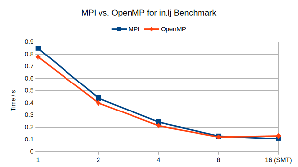
@chrisp to support my statement, here are some strong scaling numbers I just collected on my desktop with a mobile 8-core CPU with SMT enabled. This is using a tiny system with just 32,000 LJ atoms with a rather short 2.5 \sigma cutoff.
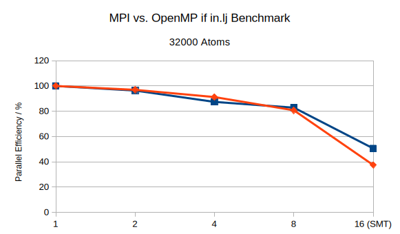
OpenMP is a little bit faster in absolute performance, since the OpenMP version of the pair style has some additional optimizations that are missing from the base style. Parallel efficiency is almost the same, only when using the SMT threads thing start to break down. In this case OpenMP works quite well because the system is so small that the data fits to more than 50% into the per-core L2 cache and all data into the global L3 cache.
Thanks a lot for the detailed explanation, it was nice clarifiyng how the communication of ghost atoms wih MPI domain decomposition works. The fact about the higher cache efficiency of smaller subdomains seems obvious but I would have never thought of it myself.
Regarding force decomposition, I understand the bottleneck imposed by communication in the general case, which is why I was referring to the particular case of noninteracting molecules. To make the situation clearer, one can imagine wanting to simulate N molecules with P available cores. As fas as I am concerned there are 2 main scenarios:
Create a simulation box with N molecules and split it into P MPI tasks (or OpenMP threads?)
Launch P independent single-core simulations, each containing N/P molecules
To my understanding, scenario 2 is going to be more efficient since no communication between subdomains is involved. But the logistical mess of having to combine the outputs of separate simulations is not very appealing, which is why I was wondering if LAMMPS has a functionality similar to scenario 2 (I don’t think so).
Finally, I’m curious as to how you calculate parallel efficiency in the second plot? I would always expect a value below 100% that drops with increasing number of cores/threads. Also given the data on execution time from the first plot I would expect that OpenMPI works worse with SMT when compared to MPI.
Your thinking is incorrect. LAMMPS can be run in multi-partition mode and you use the same input because it can have per-partition variables to augment the input with different numbers and/or you can prefix commands with the partition command to select on which partition or not it is run.
That will be the same, since the runs are independent, just on different (groups of) MPI processors.
My bad! I put this together very quickly and didn’t notice that I reversed the numerator and denominator. Here is the corrected graph. The expression is: P_{eff} = \frac{T_1}{n \cdot T_n} \cdot 100\%. The general rule is that it does not make sense to use additional parallelization if the parallel efficiency drops below 50%.
That doesn’t make much of a difference, since you still loop over only the local components, only that the neighbor list is much shorter and your forces come mostly from the bonds and from intramolecular pairs that are beyond the 1-4 exclusions. That will also likely make time integration a significant time consumer, which also is perfectly parallelized. You can also reduce in this case the burden for computing ghost atoms by reducing the cutoff. If you want to disable pairwise non-bonded computations entirely, you can use pair style zero and adjust the cutoff so that the communication cutoff is sufficient for the bonded interactions.
OpenMPI is MPI. You probably meant OpenMP (a one letter change but a big difference).
It is, and the reason for that is contention for memory bandwidth. In multi-threading each thread writes to its own copy of the force array, thus the writes have to work on nCPU times the memory, which is less efficient, while with MPI each processes has an 1/nCPU size block of the force array to work with. The SMT benefit usually vanishes with multi-node runs since then the communication device becomes the bottleneck and running MPI + OpenMP is usually the fastest and the balance between MPI and OpenMP is determined by the available communication bandwidth.
Yes but if I understand correctly, running in multi-partition mode means having discrete output files for each partition making postprocessing just a bit more annoying, not something worth complaining about though.
Well, I would not dismiss this option so quickly, you could reduce the amount of preprocessing needed by using the following steps in your input:
use reset_timestep to set the initial timestep number so that you give each run a unique range of timestep numbers
use a uloop variable and embed that value in file names using ${varname} so that each per-partition run has a unique filename and that number is aligned with the timestep number range from the previous step
use the log command to set the name of the log file according the uloop variable
with all the precautions you can combine the dump and log files in the same order with just the cat command and then post-process away.
P.S.: I forgot to mention, that you may want to use dump_modify first no to remove the “indentical” first time step before the system diverges from using different velocity initialization seeds for each partition