run.in (3.3 KB)
I calculated the thermal conductivity of n-decane using the EMD method at 600K and 3MPa, using the oplsaa.lt in the moltemplate to generate force field information. However, the difference in thermal conductivity between the calculated values and NIST is too large. NIST gave a value of 0.075052W/mk, while I calculated a value of~0.42/Wmk. In the published literature, it is roughly around~0.1W/mk. I don’t know the problem, can anyone help me?Below is my “in.file”.Thank you in advance
What you are asking for is asking quite a lot. This is not something that can be resolved by just having a quick look at your input and then giving you a “do this, not that” kind of answer.
Instead, somebody would have to rerun your simulations and do all the kind of checks that could be made to confirm which are the adequate choices for your study. In particular:
- is the method you are using suitable for the kind of system you have? there are multiple alternatives, you can try them out to see if they produce the same results or at least search the published literature to find what others have been using successfully for similar systems
- are your results converged with respect of duration of equilibration, duration of data accumulation, and system size? convergence is usually simpler for highly mobile atomic liquids.
- are your choice of force field parameters (atom type, partial changes) and simulation settings correct and can you reproduce other properties from equilibrium simulations (RDFs, self-diffusion, density, etc.)?
You are not very likely to find somebody who will do all that for you and then tell you what to do.
Since this is less a question about how to use LAMMPS but rather about how to do research, you will probably want to discuss this with your adviser or tutor or senior colleagues.
As @akohlmey said, a full scale debugging is not really possible (that’s part of your research). Note that your calculation is already within 4-6x of an acceptable value, the same order of magnitude, so you’re quite close!
If another paper has calculated a thermal conductivity you consider reliable, using the same or a very similar MD method, you should try to duplicate that paper’s result first. I can’t run any calculations, but if you put a reference here I can skim through the paper and see if there are any major differences.
If you have disk space, try to write out the velocities as well as positions next time you make a big run. That way you can reanalyse the trajectory in full and see if the problem is in post-processing.
I notice you have an npt equilibration, and you are using PPPM electrostatics. If the volume changes dramatically the old grid settings may not be appropriate (although they should be recalculated between runs – I forget, check your log files). To be safe, run two blocks of npt (perhaps each with half the time) to see if the box volume stays the same.
Last tip – find a value of the gas constant R in units of kcal/mol. Use that instead of the Boltzmann constant k_B and you save one unnecessary conversion step. It’s a small thing, but every small thing you take out of your script makes debugging easier.
Thank you for your reply. Firstly, I have read a large amount of literature, most of which use the EMD method to calculate thermal conductivity. In fact, I am repeating an example from a literature, where 600K and 3Mpa are just one of them. I am not sure if the npt set in my in.file is correct at 29.6 (3Mpa=29.6 atm?). There are also many force fields used in the literature, and opls is just one of them. No one around me knows how to use LAMMPS, and the significant difference between the simulation results and NIST data has been bothering me for a long time. I have been trying to solve it but have not achieved good results. The force field parameters directly obtained from oplsaa.lt in the template I used (lopls should be better). The steps for simulation in the literature are roughly as follows: “The EMD simulations are carried out in 3D cubic box with period.Boundary conditions applied along the x -, y -, and z directions to avoid edge effects on the bulk fluid The time step is set as 1 fs. The cut off distance for L-J interactions are chosen as RC=3.5 σ. For the simulations with all atom models, column interactions for a distance of two atoms shorter than 1.8 nm are calculated directly while that further is calculated through the particle-particle/particle mesh (PPPM) method with a precision of 10-5. The minimization of energy is carried out through the steepest descent method. The simulations initially run for 500 ps in an isochoric infrared (NVT) ensemble to control the system temperature. Then it is switched to the Isobaric infrared (NPT) and equilibrate the system at a given Pressure and temperature for 500 ps. Finally, the micro technical
Ensemble (NVE) is used and simulations run for 500 ps for relaxation, and the following 2.5 ns is used for production and output.” I also attach the literature below and my log output file. I hope you can help me. Thank you.https://doi.org/10.1016/j.molliq.2021.117478
log.lammps (225.9 KB)
Then you or your supervisor need to find a collaborator that does and cares about your research.
?
??
???
Are you using some software to translate your posts to english? If yes, you need to use a better one? If not, you will have a big problem writing a publication in any place that requires English.
I’m sorry, I made an error in copying the literature.The first one is Coulomb interaction, the second and third are NVT and NPT, respectively. Regarding the first point you mentioned, I think I am powerless.
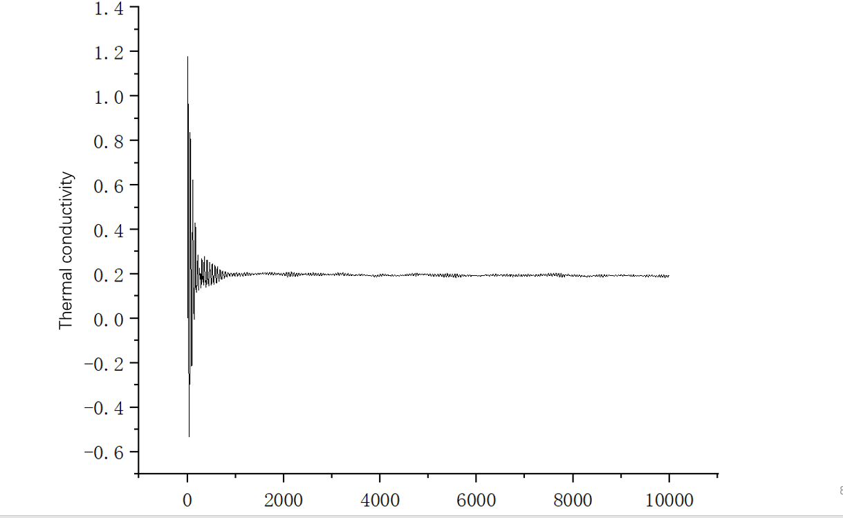
Regarding the EMD: integrating the heat-flux autocorrelation function is a bit painful, i.e. it is not easy to know what the upper integration limit should be. In theory you should “integrate up to infinity”, but as you increase the lag time in your autocorrelation function the statistical noise increases too. So, be aware of this and test it carefully. Maybe plot your thermal conductivity as a function of integration interval and inspect what happens.
1 Like
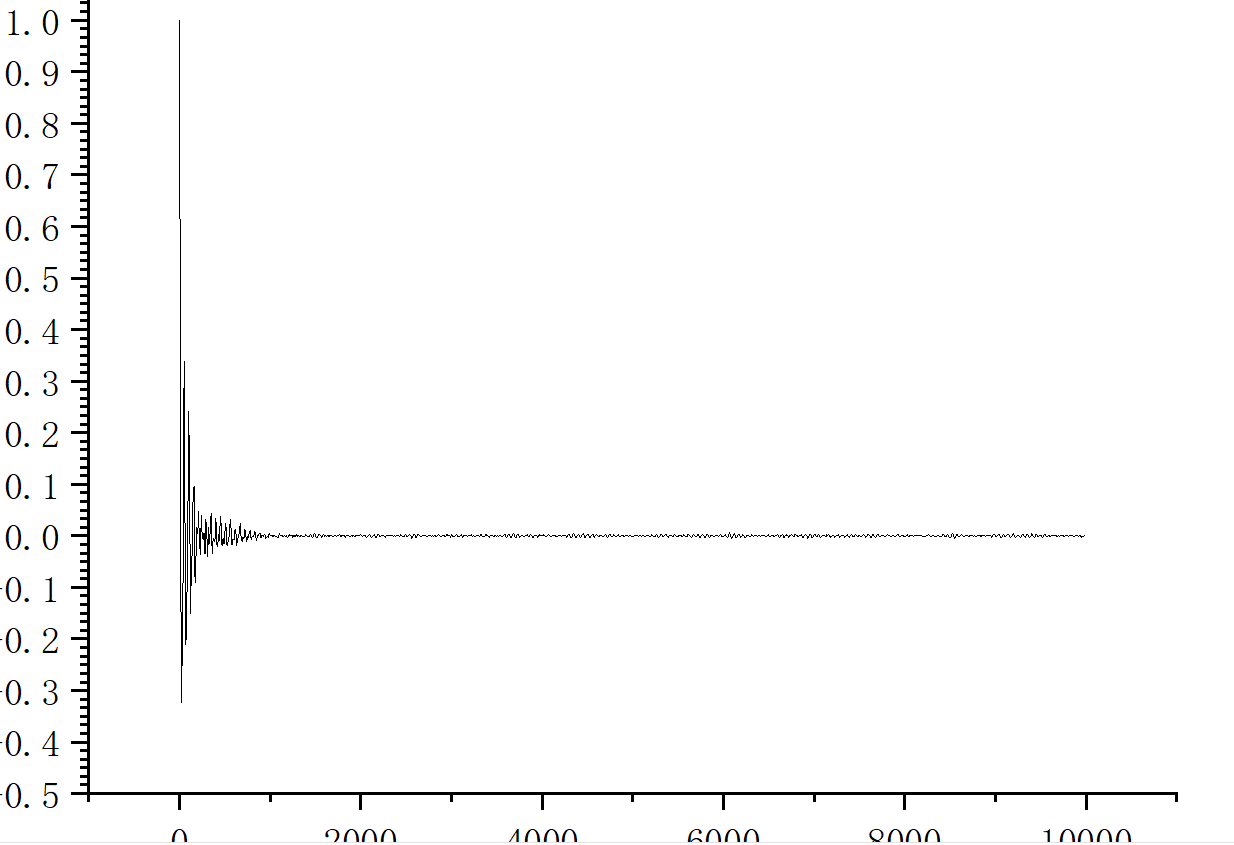
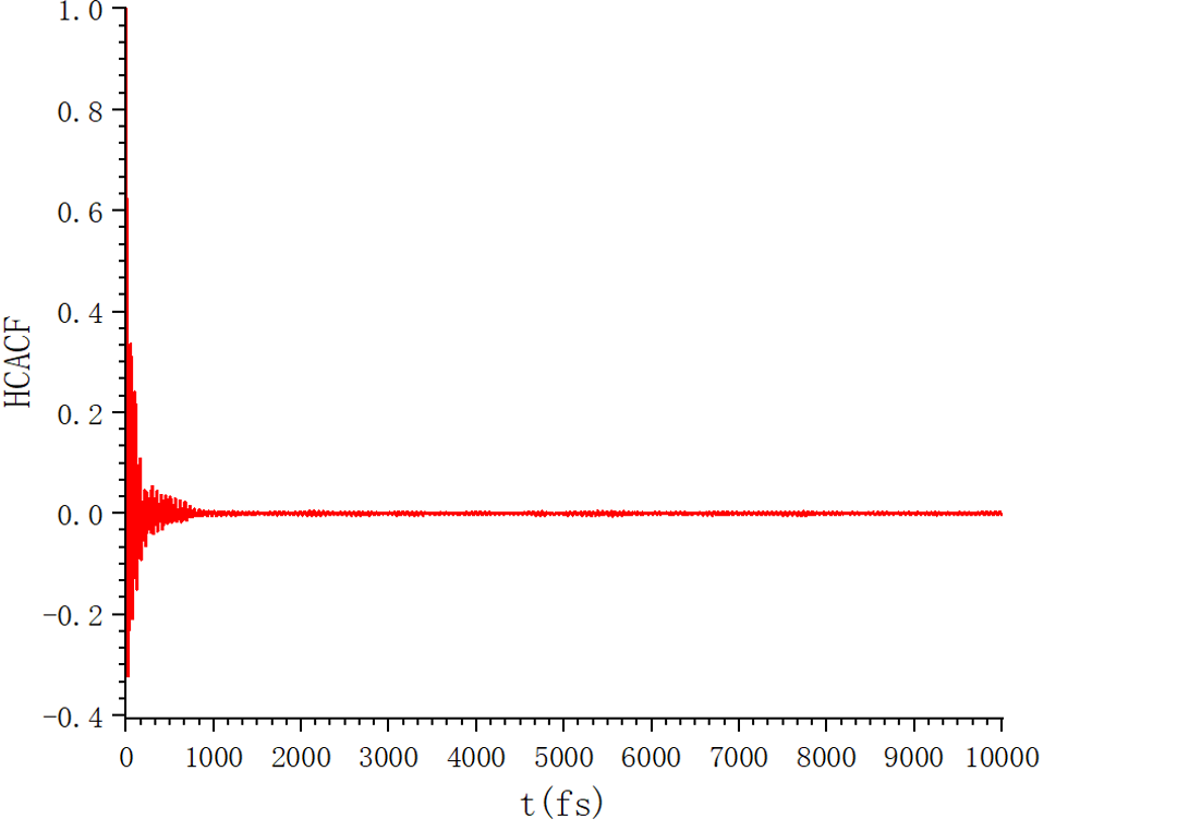
I used the values from the last window to draw the autocorrelation function vs time graph, and plotted the running thermal conductivity in the x-direction. It is obvious that there is a deviation between the data and the reference value.

Can someone give me some advice? I don’t understand why there are negative numbers in my thermal conductivity picture, is this not a normal phenomenon.
Well, you integrated an autocorrelation function which for short times has negative values. Why are you surprised? The thermal conductivity you are after must be converged which for short times you are concerned about is definitely not. As you can see from your second plot your integral did not converge yet.
Thanks,AnzeH.The negative values are normal.I checked mine data.file and found the issue.So I rerun my in.file.Acutually, this is still a big difference in the nist database and in my results, as well as in the literature. In my in.file, my s,p was changed to 5 and 2000, respectively.I also print the autocorrelation function vs time graph, and plot the running thermal conductivity.Can anyone could help with me ?I am very grateful to every teacher who has given me valuable advice.
In fact, I am not sure, for example, if I want to obtain a certain thermophysical property at 600k and 3Mpa, as described in the literature, NVT first, thenNPT ,and then NVE. So I’ll just write fix fxnvt all nvt temp 600 600 100 * dt, then fix fxnpt all npt temp 600 600 100 * dt iso 29.607 29.607 (in real units, 3Mpa=29.607atm) 1000 * dt, and then fix fxnve all nve. Is that correct? Do I need to do any other operations?