Transverse acoustic modes in S(q,w) and C(q,w)

[apoletayev]

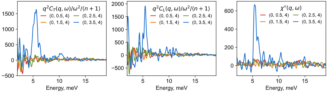
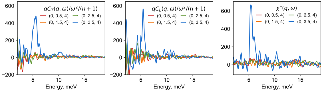
I am attempting to reproduce some of the calculations related to transverse acoustic modes in this paper (their figure 3f in particular) using dynasor. Numbered equation 1 in the dynasor 2 paper relates the dynamic structure factor to the longitudinal current correlation function exclusively: w^2 S(q,w) = q^2 C_L (q,w). I am puzzled by how the first paper claims to simulate the dynamic susceptibility for transverse modes from the structure factor. It would make sense for the dynamic scattering factor to contain both longitudinal and transverse modes, because neutron scattering probes both polarizations. I also tested the above equation from my own simulation analyzed with dynasor, and did not obtain correspondence between spectra of S and C_L versus frequency at specific q-points, although there is approximate correspondence in overall spectral shapes. In my ideal world, I would be able to reconstruct the longitudinal and transverse components of the dynamic structure factor separately. What am I missing, or what could I do to troubleshoot?

Thank you!
-Andrey

[erikfransson]

@apoletayev

It would make sense for the dynamic scattering factor to contain both longitudinal and transverse modes, because neutron scattering probes both polarizations.

Maybe yes and no depending on what exactly you mean.

Strictly speaking, transverse modes are defined as those with “motion” or displacements perpendicular to the q-vector, e.g. a mode (mode A) with q=(0.5,0,0) and atoms are oscillating in (0,1,0) direction. These are sometimes referred to “selection rules” iirc.
My understanding is that with this definition, the dynamical structure factor, S(q,w) , does not contain information about the transverse modes.
So if you have a q-point X=(0.5, 0,0) in S(q=X,w) u will only see the longitudinal modes.
See this tutorial here where you see that S(q,w) (when sampling in the first BZ) only picks up the longitudinal part.

However, in INS and also simulations you can go outside the first BZ, and e.g. look at X2 =(0.5, 1, 0), which should be “equivalent” to X. But in X2 the displacements of mode A is no longer perpendicular to q, and thus we can observe the transverse mode A (that exists at q=X).
So what you (can) do in practice is measure S(q,w) for many q-points and in many different BZ and then “fold” these back into the first BZ to construct the full phonon dispersion including transverse modes. So in that sense you can obtain information about transverse modes in the system via S(q,w)

See for example this and this paper

---

@apoletayev

I also tested the above equation from my own simulation analyzed with dynasor, and did not obtain correspondence between spectra of S and C_L versus frequency at specific q-points, although there is approximate correspondence in overall spectral shapes.

Can you attach this figure?
If u multiply S(q, w) with the omega^2 factor then atleast in my experience spectra will look very similar to C_L(q, w), ofc numerical noise etc can create differences.

[apoletayev]

Dear Erik,
Thank you for the detailed response. I really should have put together the selection rules myself, but since I did not, I appreciate that you took the time to write out an example. Some of the writing in neutron papers makes more sense now. So maybe more naively - is there an equivalent of the equation w^2 S(q,w) = q^2 C_L (q,w) for q-points outside of the 1BZ which would incorporate C_T but without an explicit summation over all lattice translation vectors that would fold other BZs onto that point?

Regarding the numerics of the correspondence between S and C_T/C_L, I simulated a structure that is similar to the structure discussed in the linked original paper, a 2 x 10 x 10 supercell with some disorder in specific sites, and lithium moving about. My simulation was 400 ps at 200 K, theirs likely a bit longer because their noise looks smaller; the Nyquist frequency is the same giving energy resolution 0.052 meV. I chose q-points as in the original paper but added the equivalent (0, 4, L) points to reduce my noise.

Anyway, I plot all quantities as dynamic susceptibilities, dividing S by <n_BE + 1>, where n_BE is the Bose-Einstein occupancy at the simulation temperature. To get the equivalent quantities from the current correlation functions, I multiply those by |q|^2 and divide by w^2, before also dividing by <n_BE + 1>.

The general features are similar enough. Strongest intensity at the (0, 3.5, 4) point because there is a phonon there approaching the allowed reflection at (0, 4, 4). The intensity in all plots is at about 6 meV, with something small at 10 meV. But the absolute numbers are off, and the correspondence is not exact. Oddly enough, if I multiply the correlation functions by |q| rather than by |q|^2, I get a better correspondence here in absolute terms:

I can also upload the output of dynasor that I used for these figures (≈ 50 MB), the jupyter notebook with the plotting, and/or put the raw trajectory on zenodo (≈ 12.5 GB). Thank you again for the time you are devoting to users like me.

[erikfransson]

Yes spectra look similar but not perfect agreement.
Since the spectra look quite noisy I think its hard to get a better agreement than this.

Regarding the absolute values of q^2/w^2 * C_L agreeing with S(q,w) or not , Im not sure if we have ever tested this properly.
There could be some factors of pi or normalizations etc that get lost.
And it would also require you to keep track of units properly, units of your velocities in your trajectory (since C_L and S and have different units and q^2/w^2 have units and so on).

[apoletayev]

Okay, thank you for the response! I admit I did think of these transformations as things that should in principle be exact starting with the same simulation data. I can see in principle how factors of pi or something like that could enter in the Fourier transform terms, but I will probably leave it at approximate agreement for the purposes of my current project.

[erikfransson]

Usually the absolute value of spectra are not very relevant and thus I think this question rarely comes up.

@apoletayev

is there an equivalent of the equation w^2 S(q,w) = q^2 C_L (q,w) for q-points outside of the 1BZ which would incorporate C_T but without an explicit summation over all lattice translation vectors that would fold other BZs onto that point?

Also sorry I missed this. Afaik there is no general equation, but if you have knowledge about your specific system and its modes then one can probably figure out which transverse mode would show up in C_L for q-points outside 1st BZ.

[apoletayev]

Yes I agree that the absolute values probably do not regularly surface. In this particular case the question of absolute values arose because the paper I was attempting to reproduce (see, e.g., their figure 3f and supplementary figure 24) argued that the intensity of a particular transverse phonon mode was decreasing with temperature. So here the intensity needed to be self-consistent between LA vs TA branches across distinct BZs and across several temperatures. A bit of a niche application perhaps