Hello everyone,
I am a beginner in using LAMMPS and currently working on a simulation of the Soret effect in an ethanol-water mixture. However, I could not reproduce the expected linear temperature gradient and ethanol concentration gradient. I would appreciate any advice or feedback on my simulation settings.
Simulation Overview
Objective: To simulate the Soret effect in an ethanol-water mixture and observe linear temperature and concentration gradients.
Conditions:
Number of molecules:
Water: 760
Ethanol: 40
Models used:
Water: TIP4P
Ethanol: OPLS-AA
Simulation box: Created using water_ethanol_box.txt
Temperature gradient: Applied using the fix langevin command
Simulation time: 1000 ns (50 million steps)
Temperature range: Applied a linear temperature gradient across the system
The molecular and parameter files for water and ethanol were referenced from Simon’s GitHub repository.
Steps Taken
Created the initial configuration using water_ethanol_box.txt.
Performed energy minimization.
Assigned initial velocities after the minimization.
Applied a temperature gradient using soret.txt and ran a 50-million-step simulation.
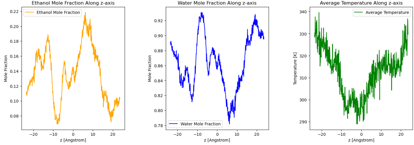
Plotted the resulting z-direction temperature and concentration profiles, as shown in 5000.png.
The data was sampled every 5000 steps and averaged over 100 samples to create the final plot.
Issues Observed
The results did not meet the expected characteristics:
The z-direction temperature gradient is not linear.
The ethanol concentration gradient is not linear.
Additionally, I tried reducing the number of bins during the data binning process for graphing, but this did not resolve the issue.
Questions
How can I modify my simulation settings to obtain a linear temperature gradient and ethanol concentration gradient?
Any suggestions or insights into possible mistakes or areas for improvement would be greatly appreciated.
you are running for 100 ns. Given that your system is 5 nm long, and given the diffusion coefficient of water-ethanol mixtures at such temperature, this may be too short to reach a properly equilibrated state.
Do you have any reason to believe that this effect (you don’t even explain what it is, so I had to google it), should manifest itself on the time and length scales of an MD simulation and particularly for a such a tiny system with only 800 molecules? The references displayed by Google all seem to refer to macroscopic experiments.
Why such a gigantic neighbor list skin? This will make your simulation extremely inefficient, since the neighbor lists will be flooded with pairs that have no interaction (remember the number of pairs grows cubic with the neighbor list cutoff, which is the sum of the pairwise cutoff and the skin distance).
region hot1 block INF INF INF INF ${Z0} ${Z1}
region cold block INF INF INF INF ${Z2} ${Z3}
region hot2 block INF INF INF INF ${Z4} ${Z5}
Why three regions? Why not either move the definitions by (zhi-zlo)*0.015?
Or create a single hot region with?
region hot union 2 hot1 hot2
compute temp_chunks all chunk/atom bin/1d z lower 0.1 units box
A bin width or 0.1 Angstrom is far too small for measuring profiles of atomic scale object. You are just inviting noise.
The temp_profile.dat data should contain 50000000 / 500000 = 100 data sets. Which one did you plot?
Given the small size of your system and the small binning width, at least the temperature gradient looks roughly as it should. What if you average over more samples or combine multiple of the data sets, say the last 20 or 50? That is the usual way to reduce noise.
As already mentioned, keep in mind that your time and length scales and thus also the temperature gradient are very different from macroscopic experiments.
Thank you for your detailed feedback on my previous question. I would like to provide additional context regarding my simulation setup and ask for further clarification.
The settings for the number of molecules, box size, neighbor list, and simulation time in my study are based on the 2005 paper by Nieto-Draghi et al., titled “Computing the Soret coefficient in aqueous mixtures using boundary driven nonequilibrium molecular dynamics”. In their work, they used the Müller-Plathe algorithm to generate a temperature gradient.
In my case, I initially intended to use the Müller-Plathe algorithm, but I encountered a limitation: the fix thermal/conductivity command in LAMMPS does not support rigid or molecular systems. As a result, I followed the approach described in the 2021 paper by Takeaki Araki et al., titled “Contribution of internal degree of freedom of soft molecules to Soret effect”, to create the temperature gradient using fix langevin.
In the study by Nieto-Draghi et al., they reported that a 100 ns simulation was sufficient to reach a steady state. My question is whether this faster stabilization is primarily due to the Müller-Plathe algorithm they employed. Specifically:
Is it inherently more efficient than methods like fix langevin or fix ehex for generating a temperature gradient?
When using fix langevin or fix ehex, would it generally require a significantly longer simulation time to achieve a comparable steady-state gradient?
Regarding the data analysis in my simulation, I plotted the temperature and concentration profiles based on the last portion of the simulation. Specifically, I averaged the data from steps 49.5 million to 50 million (the last 1% of the simulation) from the 100 datasets generated by the fix ave/chunk command.
I am seeking guidance on whether there are adjustments I could make to my current setup (e.g., simulation time, gradient strength, or sampling approach) to better align with the results reported in the literature.
Thank you again for your time and insights. I greatly appreciate any advice or suggestions you can provide.
Thank you for your observation and the clarification regarding the simulation time. Also, I would like to express my gratitude for the resources you have provided on GitHub. They have been invaluable in helping me set up my simulation and understand the parameters needed for water-ethanol mixtures.
You are correct that my input script specifies a timestep of 2.0 fs and a total of 50 million steps, which corresponds to 100 ns, not 1000 ns as I initially mentioned in my post. I appreciate you pointing out this oversight.
Given your comment about the diffusion coefficient of water-ethanol mixtures and the potential for insufficient equilibration, I understand that a longer simulation time might be necessary to reach a properly equilibrated state. Based on your expertise, I would like to ask:
In your experience, how much longer should I extend the simulation to ensure adequate equilibration for a system of this size (5 nm) and composition?
Would you recommend focusing on increasing the total simulation time, or should I also adjust other parameters, such as the temperature gradient strength or binning intervals, to improve the equilibration and sampling?
Thank you again for bringing this to my attention and for your valuable feedback. I look forward to hearing your suggestions.
The only reliable solution is to measure a relevant output from your system over time, and make sure that this output has converged before the end of the simulation. In the case of mixtures… may be the mixing enthalpy would be a good quantity to evaluate?
If you need an estimate for simulation duration before launching it, a rule of thumb for systems that are limited by diffusion is to calculate the typical time required by the molecules to explore the system, \tau = L^2 / D_s, where L is the system caracteristic size, and D_s a typical self diffusion coefficient for your system. Then, to be on the safe side, you can use a duration for the simulation of the order of 5 \tau or 10 \tau. Using D_s = 1e-9 m2/s and L = 5 nm, you get \tau = 25 ns. Note that with a duration of 100 ns, you are not so far from 5 \tau, but its possible that in the case of mixtures this estimate is wrong due to the collective effects such as molecule clusters formation.
I never tried to simulate this particular phenomena, so I can’t really help. Increasing the temperature gradient would probably help in reaching a quick equilibrium, but it would also expose your system to an even stronger gradient, which is rarely great, particularly if your goal is to connect with macroscopic experiments in which gradients are always much smaller than in MD (because of the small size of MD systems).
Thank you very much for your detailed response and insights.
Your explanation has clarified that the issue lies not in the command usage but in the system not reaching equilibrium. Based on this, I will focus on revising my simulation setup to ensure proper equilibration. This includes reviewing the simulation duration, temperature gradient strength, and other relevant parameters to align with the physical characteristics of the system.
Thank you again for your guidance. I now have a clear direction for improving my setup.