I am trying to reproduce the phase diagram of discotic liquid crystals (oblate ellipsoids) using Gay-Berne potential, but failed at the beginning to generate the isotropic phase.
My run directly go to a more orientationally ordered phase, also the internal energy/enthalpy is lower than expected. The internal energy per particle is around 90 in Busselez 2014, but mine is already negative.
I use npt/asphere to control the system under reduced unit following [2] the MD study using LAMMPS, all units and timestep are set the same.
The energy unit is directly 1 at the crossed configuration [1],also checked with two single particles using the same pair style.
Since the potential setting should be correct, I cannot tell if the NPT setting is wrong.
Please tell me which part I should fix to get the isotropic phase.
Best,
Syd
Quick script for T=12, P=100 case:
#repeat aspect ratio 0.2 with Busselez 2014
#-----------------------------------
clear
units		lj
atom_style	ellipsoid
atom_modify	first big
dimension	3

# create big ellipsoidal particles

lattice		sc 0.1
region		box block 0 16 0 16 0 16
create_box	2 box
create_atoms	1 region box

set		type 1 mass 1.0
set		type 1 shape 1.0 1.0 0.2
group		big type 1
set		group big quat/random 29890

velocity	big create 24.0 87280 mom yes loop all

# equilibrate big particles
variable        ratio equal 0.2*0.2
variable        xxx equal (${ratio}-1)/(${ratio}+1)
print           ${xxx}
variable        e0 equal (1-${xxx}*${xxx})
print           ${e0}


pair_style      gayberne/omp 1.0 2.0 1.0 2.0
pair_coeff      * * 1.0 1.0 1.0 1.0 10.0 0 0 0

neighbor	1 bin
neigh_modify	delay 0 every 1 check yes one 4000

# compute temperature and pressure, setting NPT/ASPHERE

compute         temp_trans all temp

variable        dof equal count(big)
compute         temp_rottrans all temp/asphere dof all
compute_modify  temp_rottrans extra/dof ${dof}

compute         pres_trans all pressure temp_trans
compute         pres_ke all pressure temp_trans ke
compute         pres_virial all pressure temp_trans virial

compute         p_e all pe
compute         ke_t all ke
compute         ke_r all erotate/asphere

variable        erot equal c_ke_r/4096

variable        volume equal vol

compute         orient all property/atom quati quatj quatk quatw
compute         diameter all property/atom shapex shapey shapez

# output in time average and log file

fix		1 big npt/asphere/omp temp 12.0 12.0 0.025 iso 100.0 100.0 0.025
fix_modify      1 temp temp_rottrans
fix_modify      1 press pres_trans
#compute_modify  1_temp extra/dof ${dof}

fix             3 all ave/time 1 100 100 v_volume c_temp_rottrans c_pres_trans c_p_e c_ke_t c_ke_r file temp12_0.avg

dump		1 all custom 1000 temp12_0.dump id type x y z &
                   c_orient[1] c_orient[2] c_orient[3] c_orient[4] &
                   c_diameter[1] c_diameter[2] c_diameter[3]

thermo_style	custom step c_temp_rottrans press etotal pe ke v_erot enthalpy
thermo		1000

# RUN SIMULATION

timestep        0.00025
run		500000

write_restart   temp12_0.restart
undump          1
unfix           1
unfix           3
Why is the reason for not including the kinetic energy in the calculation of the pressure? This is a tricky point in MD simulations of 3D objects, and I came up with a similar solution to yours for thermostatting and barostatting. My understanding is that the pressure for rigid bodies should include the translational component of the temperature (as you have done) and the full virial, including the kinetic energy, i.e.
compute  press_transl all pressure temp_trans
###
fix		1 big npt/asphere/omp temp 12.0 12.0 0.025 iso 100.0 100.0 0.025
fix_modify      1 temp temp_rottrans
fix_modify      1 press press_transl
Thank you for your reply.
I actually set the thermo/barostatting like this after I read another discussion topic between you and sb. on NPT/ASPHERE. Especially the temperature part should not include the rotational part of energy when controlling pressure.
for the code of compute pressure It use
If the particle is asphere, this temperature->dof term will not be 3N.
this will not be a problem when the temperature is based on translational.
But another point is that the translational temperature will only be equal to rotational temperature at equilibrium. if the system is not at equilibrium, the value of temp and temp/asphere will not be the same, which may be a problem?
In my script I use:
compute         temp_trans all temp
compute         pres_trans all pressure temp_trans
###
fix		        1 big npt/asphere/omp temp 12.0 12.0 0.025 iso 100.0 100.0 0.025
fix_modify      1 temp temp_rottrans
fix_modify      1 press pres_trans
this is the same as in your example, only the name of the compute is different, is this right?
This works for my pressure control.
When using a different setting, the npt/asphere setting in some examples
fix		        1 big npt/asphere/omp temp 12.0 12.0 0.025 iso 100.0 100.0 0.025
compute_modify  1_temp extra/dof ${dof}
It cannot (may not?) reach the target pressure and sth else went wired when I monitor the component pxx, pyy and pzz in a different simulation . So I think the translational temperature to pressure one may be better.
Yes, my bad! I overlooked your script regarding which pressure was fed to the barostat.
I don’t think this is the problem, as the thermostat will rapidly populate both degrees of freedom. Let me have a look at your simulation again and get back to you.
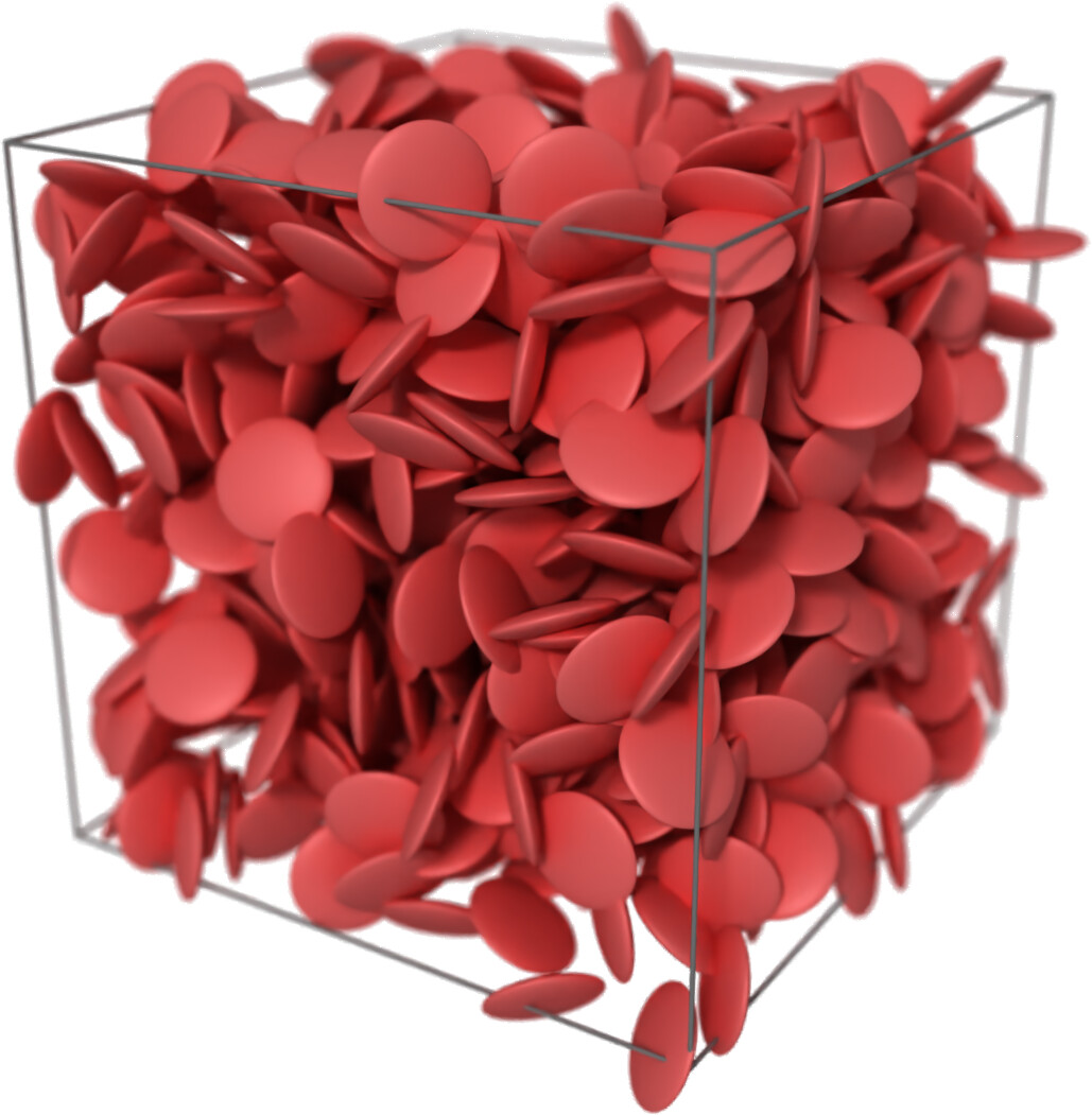
I think the problem is in the ambiguity in which the GB parameters are defined. In the papers you cited, the authors give only relative values such as k'=0.1, defined as k'=\varepsilon_\text{ee}/\varepsilon_\text{ff}. In your specific implementation, you set \varepsilon_\text{ff}=10, i.e.
pair_coeff * * 1.0 1.0 1.0 1.0 10.0 0 0 0
A more formal way to input these parameters being:
pair_coeff * * 10.0 1.0 0.1 0.1 1.0 0.1 0.1 1.0
The difference in the phase diagram arises from the depth of the potential energy well. If you set the well depth to 1.0, you get the isotropic phase at T=12* and P=100*, as you can see in the render. However, you better check a few more points in the phase diagram of Fig 10/d of reference [1].
<offtopic>
The image was rendered with Intel OSPRay, as implemented in Ovito. I have added the deep of field with an aperture of 0.4 to slightly defocus the scene. </offtopic>
Hi hothello,
Thank you for your help!
I think I did not understand the GB parameter well.
I also consult the author of reference [1], she suggest beside the ones you point out, the effective radius parameter should set to be 0.2, which is the thickness of disc particle:
pair_coeff * * 10.0 0.2 0.1 0.1 1.0 0.1 0.1 1.0
I get the isotropic phase I want with the corrected pair coefficient setting.