Different temperature/pressure behavior in small vs. large F-diamane systems using ReaxFF

aibrahim · September 12, 2025, 3:55am

Hello everyone,

I’m working on annealing simulations of fluorinated diamane (F-diamane) using LAMMPS and ReaxFF. I’ve run into some puzzling differences between a smaller and a larger replicated system, and I thought I’d seek feedback on the potential reasons behind this behavior, as I’ve viewed posts here that discuss how stable/“constant” temperature and pressure are attributed to big systems.

My work is as follows: an initial structure of an F-diamane slab with fluorine fully terminating both sides. A small system I created consisted of 384 atoms (256 C + 128 F), and I created a larger system repeating the smaller unit cell in the x- and y-directions, consisting of 3456 atoms (2304 C + 1152 F). Below is the script I use for annealing:

# 1) INITIALIZATION
# ------------------------------
variable T_start equal 10.0       # Starting temperature
variable T_end   equal 773.15     # Annealing target temperature

units real
atom_style charge
boundary p p p

read_data f_diamane_big.data

# ------------------------------
# 2) INTERACTION MODEL
# ------------------------------
pair_style reaxff NULL safezone 3.0 mincap 150
pair_coeff * * ffield.reax.FC.txt C F

# ------------------------------
# 3) GROUPS & CHARGES
# ------------------------------
group carbon type 1
group fluorine type 2
group all_atoms union carbon fluorine

fix qeq all_atoms qeq/reaxff 100 0.0 10.0 1.0e-6 reaxff

# ------------------------------
# 4) PRE-ANNEAL RELAXATION
# ------------------------------
fix boxrelax all_atoms box/relax x 0.0 y 0.0 vmax 0.001
minimize 1.0e-6 1.0e-9 1000 10000
unfix boxrelax

velocity all_atoms create ${T_start} 4928459 mom yes rot yes dist gaussian

# ------------------------------
# 5) PHASE 1: Temperature Ramp
# ------------------------------
fix temp_ramp all_atoms nvt temp ${T_start} ${T_end} 50
timestep 0.25
thermo 100
run 10000   # 2.5 ps temperature ramp

unfix temp_ramp

# ------------------------------
# 6) PHASE 2: Hold at T_end
# ------------------------------
fix anneal all_atoms nvt temp ${T_end} ${T_end} 50
fix reax_bonds all_atoms reaxff/bonds 100 bonds.reax

dump traj all_atoms custom 500 dump.lammpstrj id type x y z q
run 90000   # 22.5 ps hold at 773.15 K

# Total simulation time = 25 ps

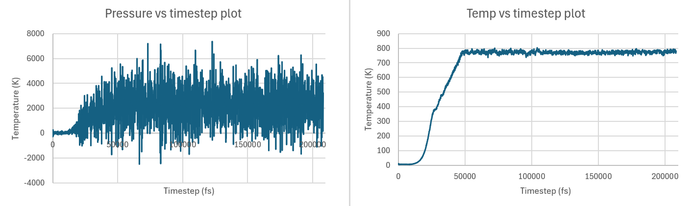
Below are the respective temperature and pressure plots for the simulation for each system:

Small system clearly showing non-convergence, and so I thought of running the same tests on a bigger system:

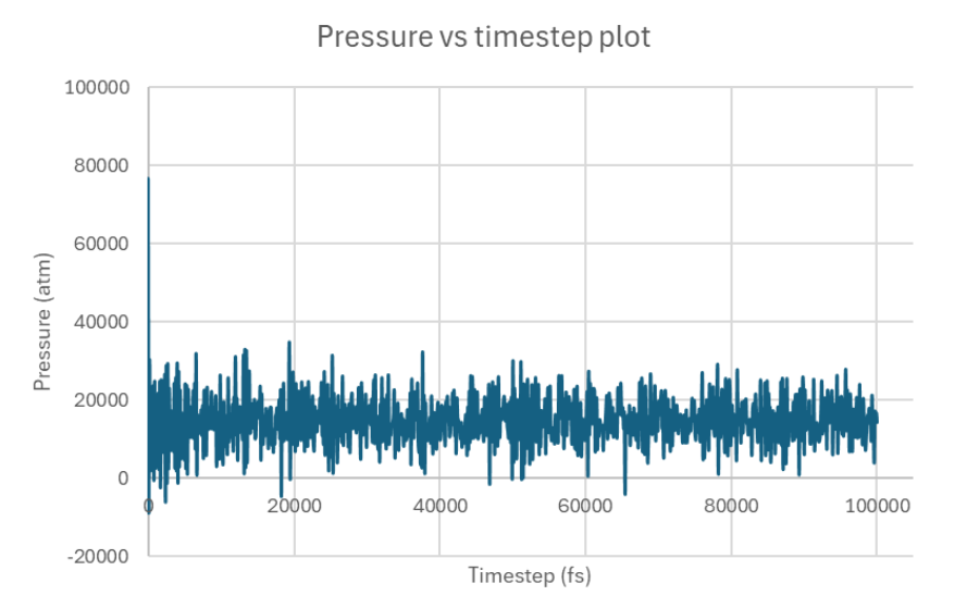
Note that the pressure plot was truncated to better display the behavior at the beginning of the run. The rest of the run exhibited smooth trends like the ones shown after the initial fluctuations.

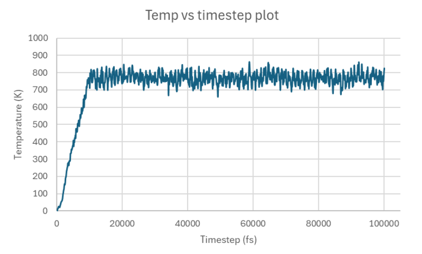
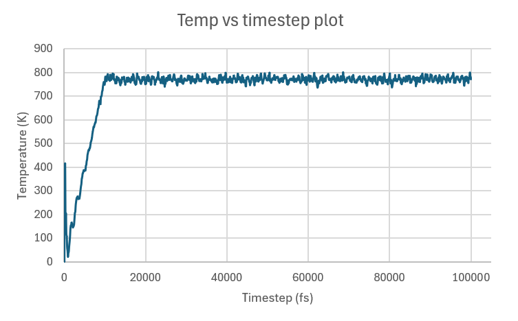
I’m happy for the most part with the temperature trends of the big system, as temperatures are more tightly packed or don’t fluctuate as much. The one concern I have is the initial temperature spike, which I believe is attributed to really high pressure:

   Step          Temp          E_pair         E_mol          TotEng         Press     
        22   10            -502971.03      0             -502868.04     -12120.994    
  -->  100   365.77929     -511393.37      0             -507626.32      48195.76     
       200   413.21375     -514338.02      0             -510082.46     -6067.4625    
       300   160.32654     -513229.38      0             -511578.22     -14845.023    
       400   204.45019     -514380.16      0             -512274.59      2087.0516    
       500   115.7196      -514030.76      0             -512839         6686.7493    
       600   106.61311     -514253.49      0             -513155.51      12875.709    
       700   60.446976     -513999.85      0             -513377.32     -34039.995    
       800   45.34627      -513956.07      0             -513489.07      19513.915    
       900   19.933844     -513774.81      0             -513569.52     -11997.832    
      1000   35.513314     -513879.51      0             -513513.77      20665.207    
      1100   43.236585     -513853.29      0             -513408.01     -41481.65     
      1200   66.191752     -513891.15      0             -513209.46      18514.136    
      1300   83.267452     -513866.3       0             -513008.76     -7292.2423    
      1400   105.54025     -513858.32      0             -512771.39      7358.7768

despite attempting to avoid this issue which I encountered with different simulations in the past by using fix box/relax to rescale the simulation box and resolve any potential in-plane strain.

Onto pressure trends, they seemed to inevitably settle down/converge but I’m curious about the cause of the initial fluctuations and if they’re attributed to my “big” system not being that big, bad practice/scripting on my part, or an alternate reason.

— LAMMPS version: 29 Aug 2024 - Update 1, on Windows

Thank you in advance and apologies for any oversights or misconceptions

aibrahim · September 12, 2025, 4:20am

Forgot to add that every run prints:

WARNING: Triclinic box skew is large. LAMMPS will run inefficiently.

My tilt factor for the respective systems (xy = 10.089 for small system, 30.266 for large system) is ~50% of the x-box length.
Not sure if this large skew is just inefficient, or if it’s affecting the stability of my runs and introducing artificial strain/instability?

Thank you

initialize · September 12, 2025, 11:19am

If you can share your full set of input files (so that others can reproduce it, ideally on a personal computer) then maybe you can get more people to help you. At the current moment I only have some general suggestions (base on the fact that E_pair drops significantly in initial steps):

make sure your minimization is actually converged (check lammps output);
check the trajectory in initial steps to see if there are large displacements;
increase the frequency of charge equilibration. Set Nevery to 1 in fix qeq/reaxff and see if it still happens.

Germain · September 12, 2025, 12:34pm

Hi @aibrahim,

In addition to @initialize comments, note that your potential energy goes down as the simulation runs. Your minimization only lasts for 1000 steps. This is very short. Are you sure your configuration reaches a local minimum before the minimization ends?

Your timestep is also in the high part of reaxff models. You might consider reducing it a bit unless you have some reference stating that this is a correct value for your model.

aibrahim · September 12, 2025, 7:36pm

Thanks for the insights @initialize, attached below are the files I’m using too:

f_diamane_big.data (300.7 KB)
ffield.reax.FC.txt (25.3 KB)

aibrahim · September 12, 2025, 8:06pm

Hi @Germain,

I only now just realized that I’ve been making the mistake of going over/taking for granted the LAMMPS output to check for the status of the minimization, but to answer your question here is the output:

OMP_NUM_THREADS environment is not set. Defaulting to 1 thread.
  using 1 OpenMP thread(s) per MPI task
Loaded 1 plugins from C:\Users\ahmed\AppData\Local\LAMMPS 64-bit 22Jul2025 with Python\plugins
Reading data file ...
  triclinic box = (0 0 -10) to (60.533997 52.423979 44.198049) with tilt (30.266999 0 0)
WARNING: Triclinic box skew is large. LAMMPS will run inefficiently. (src/domain.cpp:221)
  1 by 1 by 1 MPI processor grid
  reading atoms ...
  3456 atoms
  read_data CPU = 0.032 seconds
Reading potential file ffield.reax.FC.txt with DATE: 2013-06-28
WARNING: Changed valency_val to valency_boc for X (src/REAXFF/reaxff_ffield.cpp:300)
2304 atoms in group carbon
1152 atoms in group fluorine
3456 atoms in group all_atoms

Neighbor list info ...
  update: every = 1 steps, delay = 0 steps, check = yes
  max neighbors/atom: 2000, page size: 100000
  master list distance cutoff = 12
  ghost atom cutoff = 12
  binsize = 6, bins = 16 9 10
  2 neighbor lists, perpetual/occasional/extra = 2 0 0
  (1) pair reaxff, perpetual
      attributes: half, newton off, ghost
      pair build: half/bin/ghost/newtoff
      stencil: full/ghost/bin/3d
      bin: standard
  (2) fix qeq/reaxff, perpetual, copy from (1)
      attributes: half, newton off
      pair build: copy
      stencil: none
      bin: none
Setting up cg style minimization ...
  Unit style    : real
  Current step  : 0
WARNING: Energy due to 3 extra global DOFs will be included in minimizer energies
 (src/min.cpp:222)
Per MPI rank memory allocation (min/avg/max) = 361.2 | 361.2 | 361.2 Mbytes
   Step          Temp          E_pair         E_mol          TotEng         Press          Volume
         0   0             -497604.85      0             -497604.85      62430.708      171993.88
        22   0             -502971.03      0             -502971.03     -12147.301      178956.67
Loop time of 45.5032 on 1 procs for 22 steps with 3456 atoms

99.1% CPU use with 1 MPI tasks x 1 OpenMP threads

Minimization stats:
  Stopping criterion = linesearch alpha is zero
  Energy initial, next-to-last, final =
     -497604.845836383  -502971.026322075  -502971.026322075
  Force two-norm initial, final = 342542.92 7492.2337
  Force max component initial, final = 242162.95 2837.2084
  Final line search alpha, max atom move = 1.6412657e-16 4.6566129e-13
  Iterations, force evaluations = 22 91

MPI task timing breakdown:
Section |  min time  |  avg time  |  max time  |%varavg| %total
---------------------------------------------------------------
Pair    | 45.456     | 45.456     | 45.456     |   0.0 | 99.90
Neigh   | 0.03053    | 0.03053    | 0.03053    |   0.0 |  0.07
Comm    | 0.001656   | 0.001656   | 0.001656   |   0.0 |  0.00
Output  | 0          | 0          | 0          |   0.0 |  0.00
Modify  | 0.000108   | 0.000108   | 0.000108   |   0.0 |  0.00
Other   |            | 0.01525    |            |       |  0.03

Nlocal:           3456 ave        3456 max        3456 min
Histogram: 1 0 0 0 0 0 0 0 0 0
Nghost:           3894 ave        3894 max        3894 min
Histogram: 1 0 0 0 0 0 0 0 0 0
Neighs:         935172 ave      935172 max      935172 min
Histogram: 1 0 0 0 0 0 0 0 0 0

Total # of neighbors = 935172
Ave neighs/atom = 270.59375
Neighbor list builds = 2
Dangerous builds = 0
Setting up Verlet run ...
  Unit style    : real
  Current step  : 22
  Time step     : 0.25
Per MPI rank memory allocation (min/avg/max) = 359 | 359 | 359 Mbytes
   Step          Temp          E_pair         E_mol          TotEng         Press
        22   10            -502971.03      0             -502868.04     -12120.994
       100   365.77929     -511393.37      0             -507626.32      48195.76
       200   413.21375     -514338.02      0             -510082.46     -6067.4625

So it seems like the minimization didn’t in fact converge to a minimum. I’ll definitely give the minimization more time: minimize 1.0e-6 1.0e-9 10000 100000 and perhaps also tighten the tolerances to 1.0e-8 1.0e-10 for example?

Regarding the timestep, I’ve found timesteps under 0.5 to not be problematic with my ReaxFF work. For this specific simulation, I’ve tried 0.5, 0.25, and 0.1 but the behavior described above persisted for all of them. Not sure if that means the issue isn’t the timestep or if I should go lower.

initialize · September 12, 2025, 10:05pm

So that is the problem. Particularly note the force:
Force two-norm initial, final = 342542.92 7492.2337
The final force of 7492.2337 is pretty large and indicates that your system is far away from a “stable” configuration. And indeed you can notice large shifts of atom positions in the first steps of MD.

The real way of solving the problem should be modify your initial structure so that it is actually close to the real structure. If you just want to reach a minimum then you can try switching to a different minimization algorithm, e.g.

fix boxrelax all_atoms box/relax x 0.0 y 0.0 vmax 0.001
minimize 0 1.0e-9 20 10000
unfix boxrelax
min_style fire
minimize 1.0e-6 1.0e-9 1000 10000
min_style cg
fix boxrelax all_atoms box/relax x 0.0 y 0.0 vmax 0.001
minimize 0 1.0e-9 1000 10000

Now after minimization the force two-norm is 0.99270295 which is reasonably small, and the temperature does not skyrocket in the MD steps.

However, I have no idea if minimization in this way actually leads to a physically meaningful structure (which could only be determined by yourself).

aibrahim · November 4, 2025, 8:21pm

Hi again, thank you for your help! and apologies for the delay. I proceeded by adding the minimization steps recommended by you to my script:

# ------------------------------
# 1) INITIALIZATION
# ------------------------------
variable T_start equal 10.0       # Starting temperature
variable T_end   equal 773.15     # Annealing target temperature

units real
atom_style charge
boundary p p p

read_data f_diamane_big.data

# ------------------------------
# 2) INTERACTION MODEL
# ------------------------------
pair_style reaxff NULL safezone 3.0 mincap 150
pair_coeff * * ffield.reax.FC.txt C F

# ------------------------------
# 3) GROUPS & CHARGES
# ------------------------------
group carbon type 1
group fluorine type 2
group all_atoms union carbon fluorine

fix qeq all_atoms qeq/reaxff 100 0.0 10.0 1.0e-6 reaxff

# ------------------------------
# 4) PRE-ANNEAL RELAXATION
# ------------------------------
fix boxrelax all_atoms box/relax x 0.0 y 0.0 vmax 0.001

# 1) Quick relaxed-energy step to let box change slightly (no force tol)
#    (minimize parameters: etol ftol maxiter maxeval)
minimize 0 1.0e-9 20 10000

unfix boxrelax


min_style fire
minimize 1.0e-6 1.0e-9 1000 10000


min_style cg
fix boxrelax all_atoms box/relax x 0.0 y 0.0 vmax 0.001
minimize 0 1.0e-9 1000 10000
unfix boxrelax

# Printing final minimization diagnostics in the log (they will appear automatically).
# more informative thermo style so you can see box dims and energies during the run:
thermo_style custom step temp pe etotal press vol lx ly lz

velocity all_atoms create ${T_start} 4928459 mom yes rot yes dist gaussian

# Start recording trajectories and bonds before temperature ramp
fix reax_bonds all_atoms reaxff/bonds 100 bonds.reax
dump traj all_atoms custom 500 dump.lammpstrj id type x y z q

#short nve energy conservation test: Watch etotal/pe drift. Energy should be reasonably conserved (no explosive drift). If large drift, structure still has problems
fix test_nve all nve
thermo 100
run 8000
unfix test_nve


# ------------------------------
# 5) PHASE 1: Temperature Ramp
# ------------------------------
fix temp_ramp all_atoms nvt temp ${T_start} ${T_end} 200
timestep 0.25
thermo 100
run 40000   # 2.5 ps temperature ramp

unfix temp_ramp

# ------------------------------
# 6) PHASE 2: Hold at T_end
# ------------------------------
fix anneal all_atoms nvt temp ${T_end} ${T_end} 250

run 160000   # 22.5 ps hold at 773.15 K

# Total simulation time = 25 ps

I monitored Etotal for both the NVE run and the NVT run for phase 2 and it stayed consistent during each run, so the structure didn’t have problems as the energy didn’t drift

I then plotted the results for temperature and pressure:

The temperature is very good now, but pressure seems to still face issues with convergence, perhaps even worse than before. I’m unsure if this is due to the small size of my system or another potential cause? It looks like it started off relatively stable and then started to fluctuate much more during heating and afterwards too. I had a look at the log file and the violent fluctuation indeed starts with the temperature ramp and persists after that. The structure was also sound and remained intact at the end of the simulation and throughout it.

Are my pressure fluctuations reasonable for NVT on a slab? or should I run (fix npt) for example or switch to p p f and only barostat in-plane maybe?

Thank you again

initialize · November 5, 2025, 5:21am

There are several things you need to know:

the pressure value given by thermo output is not very meaningful if your system is not physically 3D (e.g. slabs);
the equilibrium box size at finite temperature (i.e. in MD) is generally different from the one at “zero temperature” (i.e. minimization);
the pressure value always has large fluctuations due to the limited system size in typical MD simulations (there are already lots of discussions on this topic in this forum), and this is usually not a serious problem by itself. Finite size effects does exist in MD but you should not determine its severity by the pressure fluctuations.

So due to the point 1 and 3, you should not need to worry about the pressure fluctuation itself.

However, to get a physically good simulation model, you probably need to deal with the point 2 above. This is honestly out of my knowledge (I don’t think npt is good here since the pressure output itself is not meaningful in this context). Maybe someone else with experience in similar systems can help you.

srtee · November 9, 2025, 1:44am

In your very first post you had pressure fluctuations ranging about 30,000 atm.

In your latest post the fluctuations range about 8,000 atm and include instantaneously negative values, which is typical for a solid at equilibrium at room temperature and pressure. As @initialize said, there are extensive discussions on pressure fluctuations in small systems on this forum. Not only are they normal and expected, they are related to the compressibility of your material, so you can get a rough order of magnitude of the “computational compressibility” and compare it to known values.

akohlmey · November 9, 2025, 2:23am

You should not look at the total pressure but at the components in the periodic dimensions.
For non-periodic dimensions what LAMMPS uses to compute pressure is the length of the simulation box, but this is for convenience reasons. In practice the pressure component for a non-periodic boundary is by definition 0.0 since what a LAMMPS non-periodic dimension really represents is an infinitely large vacuum around your slab.

To make it easier to see trends despite the large fluctuations (e.g. to determine if you get closer to equilibrium) people usually use fix ave/time to compute a running average over a sufficiently large window.

P.S.: BTW the y axis of your pressure vs. timestep plot is mislabeled. Also, shouldn’t the x axis be labeled “Time” and not “Timestep” or if it is the number of timesteps, then there should be no unit?

Dua_Fatima · November 21, 2025, 7:07am

Hi, this is Dua. I was doing reaxff md simulation of polymer with flame retardant to study pyrolysis and combustion. There’s confusion that when i use npt the density decreases highly but when i do nvt then pressure exceeds like crazy which approach is more realistics to study it?

akohlmey · November 21, 2025, 7:11am

This is a new topic and not related to the topic you are replying to.
Please do not “hijack” an existing discussion like this, but instead post this as a new topic with a suitable subject line.
Please see the “guidelines and suggestions” post for general recommendations on how to get the best help from the forum.

aibrahim · January 22, 2026, 10:25pm

Hi again everyone,

I wanted to ask a question about the best way for me to effectively put the slab/2D material in my simulations on a virtual substrate i.e. without actually adding substrate atoms? as that would be bad because I’m using ReaxFF which is computationally expensive. The reason I’m looking to try this is because the slab seems to be exhibiting really aggressive rippling/spontaneous curvature and eventual breakage in some cases, and we want to mitigate that.

I did some searching and I’m considering using an external potential (like a Lennard-Jones 9-3 wall) to mimic the material’s interaction with a flat surface. I have a few questions regarding this implementation:

Interaction with ReaxFF: Since I am using pair_style reaxff, is it standard to use fix wall/lj93 for example or other types of fix to apply this external force?
Parameterization: Are there established LJ parameters usedfor interactions with ReaxFF carbon/fluorine types? The specific potential I’m using is here
Thermostatting: When using this implicit wall, is there something I should look out for or change with my standard thermostat approach

For reference, here is my script’s setup section:

# 1) INITIALIZATION
variable T_start equal 10.0       # Starting temperature
variable T_end   equal 2773.15     # Annealing target temperature

units real
atom_style charge
boundary p p p

read_data f_diamane_big.data

# 2) INTERACTION MODEL

pair_style reaxff NULL safezone 3.0 mincap 150
pair_coeff * * ffield.reax.FC.txt C F

# 3) GROUPS & CHARGES
group carbon type 1
group fluorine type 2
group all_atoms union carbon fluorine

fix qeq all_atoms qeq/reaxff 100 0.0 10.0 1.0e-6 reaxff

# 4) PRE-ANNEAL RELAXATION
fix boxrelax all_atoms box/relax x 0.0 y 0.0 vmax 0.001
minimize 0 1.0e-9 20 10000
unfix boxrelax

min_style fire
minimize 1.0e-6 1.0e-9 1000 10000

min_style cg
fix boxrelax all_atoms box/relax x 0.0 y 0.0 vmax 0.001
minimize 0 1.0e-9 1000 10000
unfix boxrelax

thermo_style custom step temp pe etotal press vol lx ly lz

velocity all_atoms create ${T_start} 4928459 mom yes rot yes dist gaussian

fix reax_bonds all_atoms reaxff/bonds 1000 bonds.reax
dump traj all_atoms custom 1000 dump.lammpstrj id type x y z q

#short nve energy conservation test: watch etotal/pe drift. If large drift, structure still has problems
fix test_nve all nve
thermo 100
run 8000
unfix test_nve

# 5) PHASE 1: Temperature Ramp
fix temp_ramp all_atoms nvt temp ${T_start} ${T_end} 200
timestep 0.25
thermo 100
run 40000

unfix temp_ramp

# 6) PHASE 2: Hold temperature
fix anneal all_atoms nvt temp ${T_end} ${T_end} 250

# Write a restart file every 4,000,000 steps
restart 4000000 restart_file.R*.gz

# Write an initial restart file before the long run starts
write_restart restart_file.initial

run 20000000

Happy to provide any additional context or info needed

— LAMMPS version: 29 Aug 2024 - Update 1, on Windows

Thank you in advance and apologies for any oversights or misconceptions

akohlmey · January 22, 2026, 10:46pm

My response to this kind of argument is always that not the speed of computing resources should determine the choice of model, but the requirements of the science. If you can prove that a computationally less expensive method produces suitable results, then that is fine, but the burden of proof is on you. Please keep in mind that if you are arguing to use a “cheap” method in combination with an “expensive” method, you also have to explain why the “expensive” method is required in the first place. If you are willing to sacrifice some accuracy, why not across the whole system?

Beyond that, the argument of my computer is not fast enough is rarely sufficient, because these days it is rather easy to get access to more capable resources. Many departments and most universities have HPC clusters to which you may get access. Sometimes for a fee, but that is usually small compared to the cost of paying you for your work. Also there are regional and national supercomputing centers and there is usually some level of access where you (or your supervisor/adviser/PI) may have to submit some proposal but rarely do you get charged a fee, if you can prove the relevance of your research and that you are sufficiently competent. Many centers also provide the necessary training. Reviewers know this and thus if you write up your results in a paper and state that you chose an inferior approach because you didn’t (want to?) make an effort to get access to more capable computing resources you will just get a shrug.

These are all questions about the details of your research and not about LAMMPS. Thus it is something to discuss with an adviser, tutor, or collaborator but not in a forum about LAMMPS.
Besides, there is very little value in anybody here answering your questions since this would come from an unverifiable source, but if you need to argue the correctness of your choices you cannot state “some dude on the internet said it was ok”. Instead you have to provide convincing proof or references containing such proof and - if necessary - perform the necessary calculations yourself. Also, if you want to know if something is a common choice, you need to survey the published literature and see for yourself. Nobody will do that work for you.

Sorry if this is not the answer that you are looking for, but - as the saying goes - this is how the cookie crumbles…

aibrahim · January 23, 2026, 1:17am

Thank you for the feedback. To clarify, the ‘computational expense’ comment was poorly phrased—I am currently utilizing a university HPC cluster. My concern wasn’t just raw simulation-time, but also a limitation of the specific ReaxFF parameterization I am using, which is optimized only for C/F/H systems. Forget to mention that though, sorry for that.

Adding an explicit substrate would thus require a different potential I believe? That’s why an implicit substrate or wall seemed like an appealing approach which would also potentially maintain the integrity of the ReaxFF model I’m using.

Regarding the technical implementation, I’ll look further into the literature for LJ parameterization for these interfaces. My main goal was to confirm if fix wall is numerically stable when used alongside pair_style reaxff. Surveying the literature comes with its hurdles in my experience, as it often provides physical findings but rarely shares the underlying necessary implementation details, at least in the case of work relevant to my studies, example. This lack of available ‘best practices’ for simulating these specific materials is what made me feel like I could reach out to members of the community here who can provide insights or advice on the various approaches that I’m taking, given that I’m not a super experienced user. Thank you though for bringing to my attention the fact that as my simulations become more and more specialized or complex, the choices become more narrow and related to research than LAMMPS. When I was just getting started with LAMMPS I’d post here after reading papers and checking out resources on “best practices” to ensure that I’m building up my specialized work on a good base. My PI had minimal input in that stage as it was part of my learning experience or onboarding with LAMMPS, not yet deep in our esoteric “research realm”. As we got further along in the simulations, there became less work related to choices/methods and more analysis and input from my PI. However, when we sometimes want to resolve an issue we’re facing, or we want to look into a new method, I’m always initially wary or critical of my implementation or choice, especially if there don’t seem to be other reference points. I’m aware that this is the nature of research, and that the answers are for me to find, it’s just that I continue to grapple with the question of “is this output ok or is it bad practice on my part”, and I haven’t had much luck with getting closer to an answer to that question through literature relevant to my work. And in the cases in which I do, there isn’t enough available on what they used or did to achieve the results. I feel like becoming more autonomous/better at making that final judgement call on “is this output ok or is it bad practice on my part” is the missing piece of the puzzle for me. In my head I subconsciously viewed this forum as the reviewers or collaborative board of LAMMPS savvy experts that’ll somehow always know what’s good practice, so thank you for helping me clear that up.

akohlmey · January 23, 2026, 2:33am

Being very familiar with using LAMMPS does not mean that we are also familiar with all kinds of research. Also, if you look through the forum, you see that the number of people responding is very small. I would wish that it would be more of a community, i.e. many people offer their knowledge and experience and there are real discussion. However, the reality is rather one sided. That is OK, if people have technical problems, because even without expertise in a specific application of LAMMPS it is rather straightforward for an experience user or developer to determine how simple errors happen. However giving reliable advice on how to do a research project requires far more specific knowledge or both the field of research as a whole and the specific project and the chance to find somebody that has this knowledge readily available is extremely small. So to give a competent response requires a substantial effort. People with limited experience have a tendency to treat online forums like a genie in a bottle, i.e. if they rub it well enough, their wish will be granted.

It is rather sad that in the field of molecular simulations, the willingness to share knowledge and experience is rather limited. … and over the time of my career and as simulation tools have become more widespread and more accessible, that kind of sharing has become rather rare and the field competitive and many researchers have become very guarded to not share anything that could expose possible mistakes or lack of knowledge or would benefit the “competition” instead of their own ambitions. At the same time, the average qualification of users has declined and thus the quality of published research and thus the usefulness of (some) publications and so on. Which is a pity since we have all the great technology to sharing knowledge and building communities that were not available when I entered the field, for example. But at the time, the challenges were more of a technical nature and the complexity of research projects less (Linux was in its infancy and there were a lot of different operating systems all with their own quirks).