I am investigating energy conservation in a many-layer graphene/water system simulated in the NVE ensemble. Despite using a timestep as small as 0.2 fs, the system exhibits a gradual increase in energy (plot attached). I am using the 29th August 2024 version of LAMMPS with the Tersoff and TIP4P/2005 force fields for graphene and water, respectively.
Simulation Workflow
Step 1: Separate equilibration and validation for energy conservation in the NVE ensemble:
Graphite subsystem: Simulated for 500 ps with a 1 fs timestep.
Water subsystem: Simulated for 500 ps with a 1 fs timestep.
Observation: Energy is conserved in both subsystems during these tests.
Step 2: Combine the equilibrated graphene sheets and water slab using the read_data command:
Graphene sheets are replicated to sandwich the water slab.
Step 3: Gradual ramp-up of the timestep (from 0.01 fs to 0.2 fs) in the NVT ensemble and subsequent NVE ensemble simulation at 0.2 fs timestep.
Details and Checks
Initial Water Configuration:
Water is simulated in a fully periodic box during Step 1.
Before combining with graphene, I unwrap the oxygen and hydrogen coordinates in the x and y directions and set the image flags to 0 in the z-direction.
I verified the integrity of water by analyzing bond and angle distributions using bond/local and angle/local with ave/histo.
Alternative Configurations:
To rule out issues with the initial water configuration, I repeated the simulations using water molecules prepared via Packmol. The results remain unchanged, and energy conservation issues persist.
Attachments
Input script for the combined system (in.run).
Input scripts for individual subsystems (in.water, in.graphene).
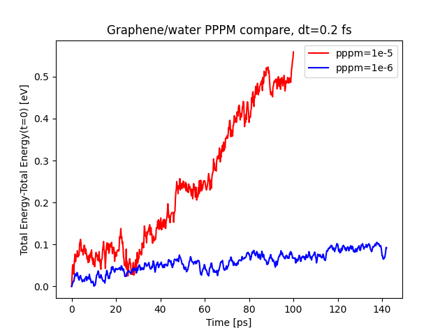
Energy plot showing the rise in energy over time.
Forcefield (in.forcefield)
This behavior is puzzling because:
Both subsystems independently conserve energy at a 1 fs timestep.
A smaller timestep of 0.2 fs for the combined system should logically ensure better stability.
I would greatly appreciate any insights or suggestions regarding the possible cause of the energy drift in this combined system. Are there known pitfalls or potential oversights when coupling Tersoff and TIP4P/2005 force fields, or when transitioning from periodic subsystems to a combined system?
Try a tighter PPPM accuracy (i.e. from 1e-5 to 1e-6 and so on).
From what I can tell, you are putting a water box of homogeneous density between two graphene pistons. This is not the equilibrated configuration, as polar layers will build up at the water/graphene interface. The resulting inhomogeneity means the PPPM accuracy may be less than its nominal estimate (which is guaranteed for largely homogeneous charge distributions) and, at the accuracy level you are tracing, this could result in very small energy non-conservation.
many thanks for your suggestion. Looks like pppm 1e-6 does the job as shown in the plot.
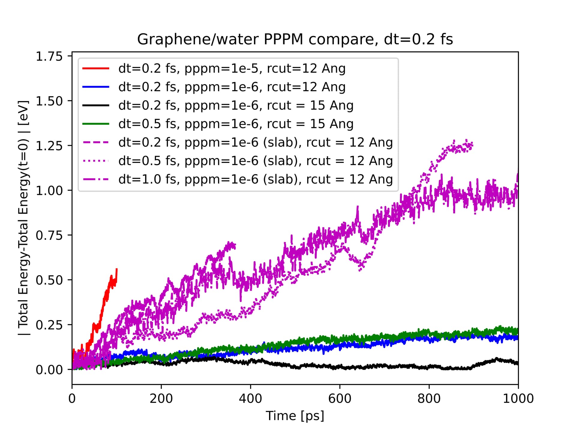
Couple of points worth mentioning. I am planning to inject and extract heat for 10 ns. The initially innocuous energy rise in the nve ensemble (without the heat flux) will no longer be negligible on the 10 ns timescale. Thus monitoring tiny drifts in the total energy is essential for my case. I plan to extend the current simulation for a duration up to 500 ps to be doubly sure that the pppm settings are perfect for my system.
an updated plot with a longer duration. There seems to be a slow drift even with a pppm accuracy of 1e-6. An even larger pppm accuracy of 1e-7 might work at a significant expense in computational costs. Thus, I suspect there might be something else at play here which I am not sensing.
Please note that by default, the coul/long pair styles approximate the coulomb interactions through tabulation. You can change the accuracy of the tabulation through pair_modify table. The default is for optimal performance.
At the moment, you can specify a tighter tolerance, but there is no value to it, because the erfc() function in real space is approximated with an expansion that is equivalent to evaluating it in single precision. You would have to change the source code to instead call erfc() from the math library instead, which has been benchmarked some time ago on Linux machines to slow down the computation quite significantly. There is a long dormant feature branch to replace the single-precision approximation with a different one that provides a better accuracy but is about as fast as the current approximation, but there is no ETA on that one.
Why not test the heat flux simulations before worrying so much about energy conservation in what’s essentially a completely different set of simulations?
Is there a way to review this dormant branch and make the necessary changes? From what I can tell, if it’s possible to gain more accuracy without sacrificing speed, it would be well worth the efforts.
I’m thinking in that direction for now. But its also worrisome because the temperature profiles from the heat flux simulations can then be quite different.
That branch will need a lot of work. It has been sitting around for a very long time (like 10 years or so). Basically, one would take it as an example and then re-implement it from scratch with the current development branch. But since it touches a lot of files, it is a lot of work and for as long as I am not getting paid properly for such kind of work, I will still to the (many) other tasks that are more pleasant to work on or take less time and effort for very little gain (next to nobody is complaining that Coulomb is not more accurate in LAMMPS and there easily 10s of thousands of LAMMPS users).
The water-graphene interface will build up significant dipole density, and your input script does not look like it uses a slab correction in the non-periodic direction. The resulting dipole-dipole coupling across periodic images is a significant collective long-range interaction. You should try repeating your calculations with slab correction to look for improvements in energy conservation.
You may also want to try zeroing the linear and angular momentum of both the water and graphene groups independently (using the velocity ... zero linear / angular options) before starting the NVE run. Intuitively, a system with (box-)stationary and mobile components in relative motion will have worse energy conservation (handwave, friction, something something dissipation).
I’ve now plotted now a bunch of cases experimenting with larger timesteps and different electrostatics settings (ppf+kspace_modify slab 3.0 and fully periodic boundaries ppp).
I’ve now zeroed the excess linear and angular momenta of the graphene sheets and the water slab separately, before beginning my nve run.
Plot below suggests energy conservation seems to be best for the case with fully periodic boundaries and with a pppm accuracy of 1e-6 and a timestep of 0.2 fs along with a 15 Ang. rcut. I don’t quite understand why the pppm slab configuration compares badly to the fully periodic case, with regards to energy conservation.
Worth mentioning that the total energy keeps rising even after 1 ns for the last case - 1 fs timestep, slab configuration, and rcut 12 Ang. I did not try 15 Ang because of the excessively slow computations.
This is now well outside my expertise. A few comments:
The high sensitivity to cutoff suggests that the energy conservation problems may well come from the LJ portion of the interaction. Try using shift yes to make the LJ energy exactly zero at the cutoff and see if that makes a difference.
See this post on the mirrored cell for a general strategy used to simulate asymmetric inhomogeneous interfacial systems, without needing slab corrections or generally non-periodic boundary conditions.
Other than that, LAMMPS now seems to be doing just what you’d expect (better energy conservation at shorter timesteps and with longer cutoffs) and this is now firmly a scientific discussion, not just technical.