Mysterious attraction between hard spheres with pair lubricate

Hello all,

I am attempting to simulate equilibrium (i.e., quiescent) monodisperse hard-sphere fluids using the Fast Lubrication Dynamics (FLD) treatment of hydrodynamics, where I am overlaying purely-repulsive 48-24 Weeks-Chandler-Andersen potentials (to approximate the hard-sphere interactions) on top of lubricate/poly and brownian/poly pair-styles. (Here, I am using ‘poly’ because I want to generalize in the end to ternary systems; for now the three species all have sigma=1)

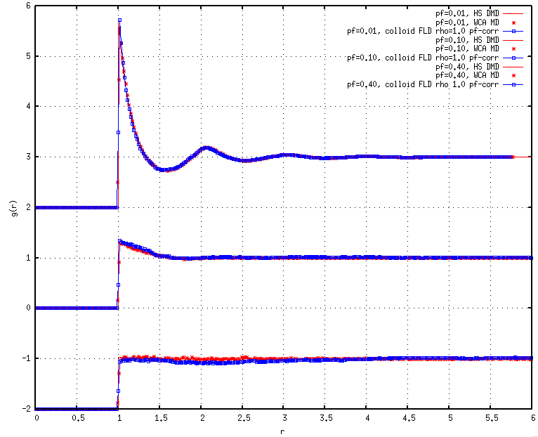
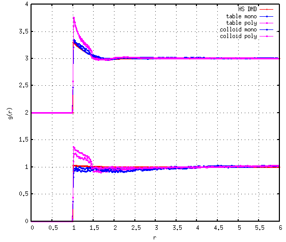
As I began to test these HS systems at different moderate packing fractions, I noticed that the radial distribution functions (RDFs) did not match previous results for WCA fluids obtained using NVT MD, instead exhibiting stronger contact values and signatures that seemed to be shifted upwards for the first and/or second coordination shells, perhaps indicating net attractions.

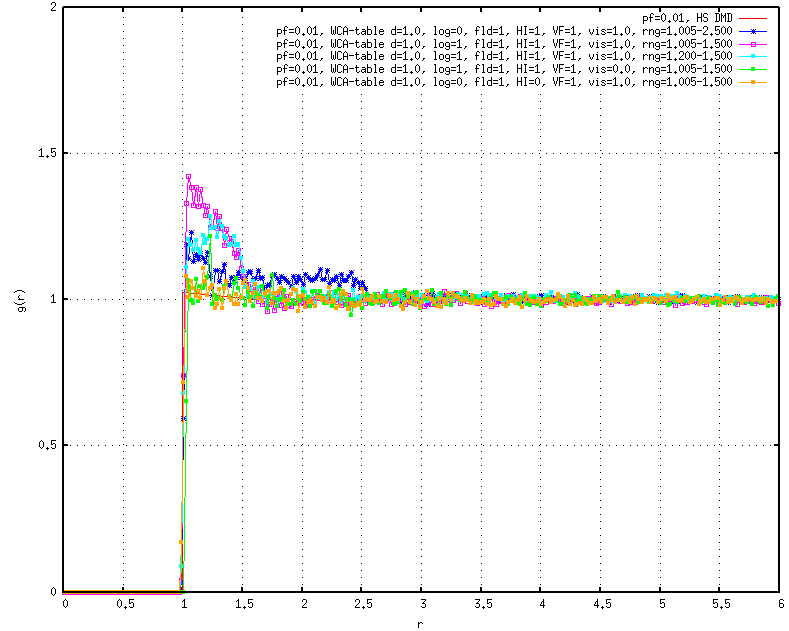
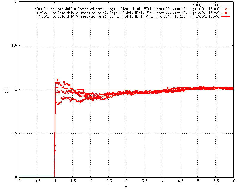
In turn, I decided to simulate a low-density system (packing fraction = 0.01), which should exhibit a step function RDF in equilibrium. Instead, I find that there are net attractions (indicated by peaks in the RDFs) between the inner and outer cutoffs of the lubrication interactions, which I have confirmed by trying different combinations of cutoffs (1.001-1.500, 1.200-1.500, 1.300-1.500, 1.001-2.500, etc.). These are not small effects, either–e.g., using cutoff 1.001-1.500, I get a contact value at r=sigma of 1.5, a peak that then decays completely by just outside of 1.500.

These effects emerge whether flaglog is turned on or off (i.e., including or excluding the Ball and Melrose log-terms), though the “attractions” are stronger when flaglog in turned on. In all cases I have tried, I have kept flagFLD, flagHI and flagVF on.

At this point, I’m a bit at a loss. Even given I am misusing the FLD commands (or even if there is a bug), I would tend to expect depletion deviations rather than attractive. Visualizing the systems does not point to anything fishy, and I should note that the RDFs do not point to any particle overlaps.

Has anyone had an issue like this previously? Any guidance/ideas would be greatly appreciated.

Details: I am using lammps/2014_01_10 run in parallel on 16 processors. Input files are listed below:

units lj
dimension 3
boundary p p p
atom_style sphere
newton off
communicate single vel yes

pair_style hybrid/overlay lubricate/poly 1.0 1 1 1.005 1.500 1 1 brownian/poly 1.0 1 1 1.005 1.500 1.0 42115 1 1 table spline 1500

read_data file.data
neighbor 0.2 bin

pair_coeff * * lubricate/poly
pair_coeff * * brownian/poly
pair_coeff * * table wca.table WCA 1.20000

thermo_style custom step xy temp ke pe etotal press
thermo 1000

timestep 0.0002
fix 1 all nve/sphere
dump xtcdump all xtc 1000 out.xtc
dump_modify xtcdump precision 100000
restart 1000000 restart.*
log log.lammps
run 1000000
unfix 1

Along with the file.data:

[comment line]

1200 atoms

3 atom types

0.0 38.51197 xlo xhi
0.0 38.51197 ylo yhi
0.0 38.51197 zlo zhi
0.0 0.0 0.0 xy xz yz

Atoms

1 1 1.0000 1.9099 15.0300 24.6310 31.6730
2 1 1.0000 1.9099 38.2340 30.3260 6.5280
3 1 1.0000 1.9099 18.9990 7.8190 32.7410

1200 3 1.0000 1.9099 31.2680 29.4610 17.0900

WCA potential file not including for now for length’s sake–rest assured I checked to ensure it is correct.

Before getting into the particulars of data and models. Have you actually checked and analyzed forces between particles (do they give what you expect given the superposition of forces), or are you just inferring everything from RDFs. You will find that an RDF for a hard sphere system is emphatically not a step function, even at 0.01 volume fraction. (try out N. Carnahan and K. Starling, “Equation of State for Nonattractive Rigid Spheres,” Journal of Chemical Physics 51, 635–636 (1969). for a commonly used estimate)

Even though 1.5 is a substantial peak, there is so much that could be going on that diagnosis of whether there is a problem via RDFs is an quite unsavory proposition. Nonetheless, post-processing is your friend here.

(Also its not particularly surprising that inclusion of FLD would give higher peaks)

Hi Eric,

I have not in-depth analyzed the breakdown of forces between particles, and am curious what you might suggest in particular, either with regards to analysis commands and/or signatures that might be telling.

Regarding the hard-sphere RDF aspect–certainly it will not be a perfect step function, but it ought to be quite close (I’m not sure what you mean by “emphatically” different). Nonetheless, I have worked extensively with hard-sphere and pseudo-hard sphere systems (in MD, at least) and can assure you that these RDFs are incorrect.

Given I’m simulating these systems at quiescent conditions, the RDFs should reflect equilibrium, no? FLD simply affects the dynamics of the system, while the conservative interparticle forces drive structure. Under shear, of course, things get more interesting.

Thanks,
J

In terms of commands, there’s nothing wrong with the regular old compute pair/local.

Keep in mind that this is not fix viscous (these dissipative forces have a spatial structure), FD does not (necessarily) apply. Look into MH Ernst’s work if you are interested in the implications.

An easy example of this is to give is a fairly dissipative granular system with Brownian forcing, you get dynamic heterogeneity. Things aren’t always as simple and straightforward as they seem. :slight_smile:

I’m CCing two folks at Sandia who have used the FLD potentials
in the past - they can comment on your Qs and input script.

I suggest not using the “poly” variants to begin with, but just
the monomeric versions. Also we typically use pair_style colloid
as the core pairwise term, not a tabulated WCA.

Steve

Thank you for the timely replies, Eric, and thank you Steve for passing this along.

Eric: in your latest email, should “FD” read “FLD”? Just want to make sure there isn’t yet another acronym out there… What do you mean by the statement “it doesn’t apply”?

Meanwhile, it’s not obvious to me in reading about FLD that it imparts/implies anything in particular about the solvent structure. Obviously, in a real suspension, the solvent possesses molecular-scale structure, the effective forces of which we’re trying to include… but again, I’m under the impression FLD treats the solvent as a structureless continuum in terms of the simulation. If I’m mistaken about this, can someone point me to the relevant portions of, e.g., work from Higdon’s group or others?

Steve: I will try implementing a monodisperse system with ‘colloid’ conservative interactions exactly resembling your previous work (from, e.g., Bolintineanu 2014) to cover bases. However, looking forward, I do hope that it will possible to incorporate tabulated potentials for polydisperse systems.

I’m very interested to hear from you and/or the folks at Sandia that you’ve added to the thread. I’m really pleased by the responsiveness on this question so far and appreciate the guidance; thanks to y’all for putting in the time.

Jonathan,

I miss-spoke (meant Fluctuation Dissipation theorem), what is correct is H-Theorem.

I am not referring to anything regarding solvent structure. I am just saying that interparticle dissipative interactions don’t always behave how you would expect. And things we know about “equilibrium” do not necessarily apply.

Here is a good example (http://journals.aps.org/pre/abstract/10.1103/PhysRevE.65.011303) and below is a good example I found recently.

Apologies for the long-windedness - but looking at forces, velocities, and positions is your only hope at really saying anything is wrong with model implementation. If you find something; I’d be interested.

DPD-KineticTheory.pdf (309 KB)

Hi Jonathan,

We’ve never seen the behavior you’re describing when using FLD with various colloid potentials, I’d be interested in tracking this down. I suspect it may have something to do with the WCA tabulated potential or the way it’s interacting with pair lubricate.

Just to clarify, you’re always seeing a peak in g® that extends between the FLD inner and outer cutoff distances?

One other quick test you may want to try in addition to what Steve suggested is to turn the FLD viscosity way down (even 0) and see what that does to the g® peak. This would at least tell you for sure that it’s FLD causing it.

-Dan

Hi Jonathan, some answers below:

Best,

Jeremy

One last more useful note.

Building on what Steve suggested (use monodisperse to start):
Is there a reason you are using both brownian and lubricate pair styles (I believe one just adds noise)?
I believe (Steve or someone else can correct) that forces and velocities are reported at different steps in the code (half step velocity used in the full step force). If that is the case, the best place to start would be to turn off any random terms (don’t know if you can set target temp to 0 and just get back pair/style lubricate), and decrease the time-step to minimize errors in calculation consistency. >From there just run a consistency check between force computes and the system configuration data that you have.

If forces and velocities are consistent, then you can even use with noise.

Hope that helps.

Hi all,

Dan: yes, that is indeed what I see. I can provide RDFs if needed. The features certainly look… stark and “unphysical”, e.g., weird plateaus near the cutoffs. I performed a run included the ‘lubricate’, ‘brownian’, and WCA interactions but with viscosity=0.0 and get back a near step-function for g®, as would be expected for HS.

Jeremy: I chose the WCA potential as a straightforward way to prevent overlaps.

Regarding the apples-to-apples/apples-to-oranges comparison: I’ve been under the impression that introducing the hydrodynamic interactions should (in the absence of shear) affect dynamics only, but not pair structure, where the latter should emerge by virtue of the conservative interparticle forces alone. (This line of reasoning arises from considering that one obtains equivalent pair structure using MC, MD, Langevin, overdamped Langevin (“Brownian”), etc. … and such results for HS in turn really nicely match pseudo-HS structure obtained from experiments). Am I just plain wrong about this? and if so, how should I be thinking about this differently?

Eric: I’m overlaying ‘brownian’ on ‘lubricate’ as the LAMMPS manual suggests this is a useful way to thermostat. As Jeremy alluded to above, I’m looking to replicate results derived from Brownian Stokesian Dynamics, e.g., ASD-nf.

I’m starting to wonder if this is a lengthscale issue? In other words, somehow ‘lubricate’ needs the colloid particles to be literally much larger than some effective solvent (riffing on the ‘colloid’ pair_style here), so maybe particles with diameter=1 are problematic?

As Jeremy (and I with the fix viscosity comment) alludes to is that although noise is uncorrelated, interparticle dissipation, which depends on the directly on the configuration of particles in physical and velocity space (unlike ordinary Langevin systems where interparticle components are conservative), can correlate random inputs through system dynamics producing structure. The essence of my side comments is that minimization of free energy is not a guarantee in the majority of these systems. In fact, it is only satisfied under special circumstances.

Jonathan,

I will do that.

Meanwhile, I’ve been going back and forth between using ‘colloid’ and trying to incorporate similar tabulated potentials. Have some new thoughts and questions that I will share after some more tests.

Thanks,
J

Hello all,

Apologies for the following novel:

Attached are two plots showing various pair structure at packing fraction = 0.01, and an additional plot showing some different packing fractions.

The first shows the RDFs that result when using a tabulated 48-24 WCA potential (d=1.0) with various combinations of lubricate+brownian settings. One can see that by either setting viscosity to zero, or turning off the lubrication terms (flaglog=0; flagHI=0), one obtains RDFs that match, e.g., MD results. However, introducing some or all of the Ball/Melrose terms at a normal viscosity results in odd, seemingly attractive features.

I also doubled-back to try and reproduce results from Bolintineanu Comp. Part. Mech. 2014. In the second plot, I include RDFs from using ‘colloid’ (d=10.0) to show that there are indeed deviations from MD HS behavior, but that these deviations are distinct from those that emerge when using the tabulated potential. (In executing the ‘colloid’ work, I picked various densities for the particles; it wasn’t really obvious to me what precisely was used in the study, so I picked a general range to see qualitative impact.) The third plot is included simply to show that the pair structure matches nicely at higher packing fractions, despite some of these depletions that emerge at pf=0.01.

Regarding the ‘colloid’ work, I have the following question: a diameter of 10 was used in defining the interparticle potential, but as far as I can tell this results in an effective particle diameter of ~10.5. Meanwhile, the lubrication interactions are set to span ~10-15 (and, accordingly, the particle diameters in the .data file are also set to 10). Doesn’t this create a mismatch? In other words, is the singularity in the HI terms getting placed at rij=10, meanwhile–particles can’t get closer than rij=10.5? How was this particular ‘overlap range’ between the two picked?

Below are the two different types of input scripts–the first for trying to incorporate a tabulated WCA potential for particle diameter=1.0 (incidentally, still using ‘poly’); the second using ‘colloid’ with the diameter=10.0 (effective d=10.5):

#################### script for running tabulated WCA system
units lj
dimension 3
boundary p p p
atom_style sphere
newton off
communicate single vel yes

pair_style hybrid/overlay lubricate/poly 1.0 1 1 1.005 1.500 1 1 brownian/poly 1.0 1 1 1.005 1.500 1.0 42125 1 1 table spline 1500
read_data datafile.data
neighbor 0.2 bin
pair_coeff * * lubricate/poly
pair_coeff * * brownian/poly
pair_coeff * * table wca.table WCA 1.20000

thermo_style custom step xy temp ke pe etotal press
thermo 1000
timestep 0.001
fix 1 all nve/sphere
dump xtcdump all xtc 1000 xtcfile.xtc
dump_modify xtcdump precision 100000 precision
run 1000000
unfix 1

#################### script for running ‘colloid’ system
units lj
dimension 3
boundary p p p
atom_style sphere
newton off
communicate single vel yes

pair_style hybrid/overlay lubricate 1.0 1 1 10.001 15.000 1 1 brownian 1.0 1 1 10.001 15.000 1.0 42118 1 1 colloid 10.0
read_data datafile.data
neighbor 0.2 bin
pair_coeff * * lubricate
pair_coeff * * brownian
pair_coeff * * colloid 39.478 1.0 10.0 10.0 10.5673

thermo_style custom step xy temp ke pe etotal press
thermo 1000
timestep 0.01
fix 1 all nve/sphere
dump xtcdump all xtc 1000 xtcfile.xtc
dump_modify xtcdump precision 100000 # make the xtc file have the desired precision
run 2000000
unfix 1

pf-0.01-lubricate-table.png

pf-0.01-lubricate-colloid.png

pf-var-lubricate-colloid.png

For the WCA simulations. What happens if you make the outter cutoff twice as big? Seems that the “overshoot” in g® decreases as outter cutoff gets bigger. For small volume fractions this is more of an issue since particles are well separated and only seldom come in and out of range But the effective impulse they feel could be large depending on the relative velocity (set by the temperature) and inverse of the separation distance. Best way to guarantee that force goes smoothly to zero for arbitrary relative velocity is have large separation distance…

Jeremy

Hi Jeremy,

That decrease in the overshoot is not solely due to the larger cutoff; that is also because I turned off the log (i.e., flaglog=0) terms in that run (leaving only the dominant squeeze HI term).

I note that the manual suggests one should use a cutoff of 1.5d when flaglog=1, but also note that Bybee/Kumar/Higdon use a cutoff of 2.5d when they ignore those log terms. Given the small pf, I imagine it will be negligible cost to actually incorporate the log terms even given an extended cutoff.

I will try to get to a more thorough set of cutoff combinations… perhaps doing 2.5d and 4d.

J

Hello all,

I have pinpointed that the “unphysical” attractions occur only upon trying to use pair lubricate/poly and brownian/poly.

To wit, the attached plot shows that using pair lubricate and brownian, one can use either ‘colloid’ or a tabulated potential (in both cases, true diameter d=10.0; effective diameter due to repulsive potential d’=10.5) and obtain essentially correct pair structure. These systems essentially replicate the setup of Bolintineanu 2014. Note that I am using flaglog=1, fld=1, HI=1, and VF=1, with lubrication cutoffs of 10.001 (inner) to 15.000 (outer).

However, when calling lubricate/poly and brownian/poly, but keeping all the particles the same diameter (i.e. system is still monodisperse in actuality), one obtains the strange structural features within the range of the lubrication forces.

Does anyone have some guidance about how to proceed? Considering the only change has been to call /poly, I consider this a potential bug, and one that makes it impossible to do poly-disperse systems.

Thanks much,
Jon

LAMMPS-FLD-colloidtable-monopoly.png

Great! Good sleuthing, looks like you are well on your way to solving the issue. Seems like the next step is to look at the code for pair_lubricate and pair_lubricate_poly and find the offending bit in the a_sq term.

Happy coding,

Jeremy

Jonathan,
I have a modified version of FLD that I’ve used for a number of studies, including some debugging/changes I had made to pair lubricate/poly that might fix this problem. One other significant change is that the pair lubricate/poly cutoffs are entered as multiplicative factors for the radii, rather than absolute values. This makes it easier to deal with arbitrary polydispersity, so that you don’t have to use a different atom type for each particle size. But it does potentially break any older scripts that are based on the original definition of cutoffs.

I can send you the code and work with you to debug and test it a bit. With Steve’s blessing, we could then update the current FLD package? Just worried about the issue with breaking older scripts though…

-Dan